For this example, we will use metabarcoding data, specifically 16S for bacteria and 18S for fungi.
The data is taken from:
First, Let’s call the MicroBioMeta package:
Let’s call other packages needed:
tidyverse is used
for all the data wrangling and visualizations and qiime2R for
calling .qza objects as output from QIIME2.
Then, Load the data and reformat. Notice the data we are loading came
from processing in QIIME2
, so the read_qza function is used to import this data into
R, also we could export the data within QIIME2 and then import the
data as .txt.
First, Let’s call all raw data:
bacteria_table <- qiime2R::read_qza("../man/Data/dada2.200.trimmed.single.filtered.cleaned.qza")$data %>% as.data.frame()

fungi_table <- qiime2R::read_qza("../man/Data/merge_table_240_noplant_filtered_nous.qza")$data %>%
  as.data.frame()

bacteria_metadata <- read.delim("../man/Data/FINALMAP.txt", check.names = F) %>% rename(SAMPLEID =`#SampleID`) %>%
  filter(Month == "2") %>%
  mutate(Treatment = factor(
    case_when(
      Treatment == 1 ~ "TC",
      Treatment == 2 ~ "TD",
      Treatment == 3 ~ "TED",
      TRUE ~ as.character(Treatment)
    ),
    levels = c("TC", "TD", "TED")
  ))%>%
  mutate(Type_of_soil =
    case_when(
      Type_of_soil == "Rizosphere" ~ "Rhizosphere",
      Type_of_soil == "Non-rizospheric" ~ "Bulk soil",
      TRUE ~ as.character(Type_of_soil)))

fungi_metadata<- read.delim("../man/Data/FINALMAP18S.txt", check.names = F)%>% rename(SAMPLEID=`#SampleID`)%>%
  mutate(
    Treatment = factor(
      case_when(
        Treatment == 1 ~ "TC",
        Treatment == 2 ~ "TD",
        Treatment == 3 ~ "TED",
        TRUE ~ as.character(Treatment)
      ),
      levels = c("TC", "TD", "TED")
    )
  )%>%
  mutate(Type_of_soil =
    case_when(
      Type_of_soil == "Rizospheric" ~ "Rhizosphere",
      Type_of_soil == "Non-rizospheric" ~ "Bulk soil",
         TRUE ~ as.character(Type_of_soil)))


taxonomy_bacteria <- read_qza("../man/Data/taxonomy_dada2.200.trimmed.single.seqs.qza")$data %>%
  as.data.frame() %>% rename(taxonomy = Taxon) %>%
  dplyr::select(-Confidence) %>%
  column_to_rownames(var = "Feature.ID")

taxonomy_fungi <- read_qza("../man/Data/taxonomy_blast_240_0.97.qza")$data %>% as.data.frame() %>%
  rename(taxonomy = Taxon) %>%
  dplyr::select(-Consensus) %>%
  column_to_rownames(var = "Feature.ID")
Then, Let’s filter and manage data. It is a good practice to use table and metadata that contains de same information and samples and in the same order.
For bacteria:
samples_bac <- bacteria_metadata$SAMPLEID[
  bacteria_metadata$SAMPLEID %in% colnames(bacteria_table)]

table_bacteria <- bacteria_table[, samples_bac]

metadata_bacteria <- bacteria_metadata[
  bacteria_metadata$SAMPLEID %in% samples_bac, ]
and for fungi:
samples_fun <- fungi_metadata$SAMPLEID[
  fungi_metadata$SAMPLEID %in% colnames(fungi_table)
]

table_fungi <- fungi_table[, samples_fun]

metadata_fungi <- fungi_metadata[
  fungi_metadata$SAMPLEID %in% samples_fun,
]
Pre-processing data
In order to use the data as input for functions of
MicroBioMeta should be in a biom format with
the column of taxonomy at the end.
In case your data is not in a biom form, we could use
the merge_feature_taxonomy function to set the data in this
format. This format will allow the use of taxonomy identity without load
another object into R.
table_bac <- merge_feature_taxonomy(table = table_bacteria,
                                    taxonomy = taxonomy_bacteria)
## Warning in merge_feature_taxonomy(table = table_bacteria, taxonomy =
## taxonomy_bacteria): 83 taxonomy IDs are not present in the table and will be
## excluded from the result.
table_fung <- merge_feature_taxonomy(table = table_fungi,
                                     taxonomy = taxonomy_fungi)
## Warning in merge_feature_taxonomy(table = table_fungi, taxonomy =
## taxonomy_fungi): 17 taxonomy IDs are not present in the table and will be
## excluded from the result.Composition exploration
MicroBioMeta has several functions to explore
composition, taxonomic identity, and abundance. Let’s explore each of
them.
Abundance barplots
Abundance barplots are useful to identify patterns in community
composition based on taxonomic identity.
This function generates stacked barplots of relative abundances using an
abundance table and a metadata file as input.
The taxonomy_db parameter specifies the taxonomic
reference database used for taxonomic assignment (e.g., SILVA, GTDB,
UNITE).
The x_col parameter indicates the column in the metadata
used for grouping samples along the x-axis, while facet_col
defines the metadata column used to split the plot into facets.
The level parameters allow us to choose the taxonomic
level to collapse.
The top_n_groups controls the number of most abundant
taxa displayed in the barplot.
If add_remain = TRUE, the relative abundances are
completed to 100% by adding a gray category representing the remaining
taxa not explicitly displayed; if FALSE, only the selected
taxa are shown.
The label parameter defines the legend title displayed in
the plot.
Finally, when save.table = TRUE, the function also
returns a table containing the relative abundances (percentages) used to
generate the plot.
abundance_barplot(table = table_bac,
                  metadata = metadata_bacteria,
                  taxonomy_db = "silva",
                  level = "phylum",
                  top_n = 15,
                  x_col = "Type_of_soil",
                  facet_col = "Treatment",
                  add_remained = TRUE,
                  label =   "Phylum",
                  save_table = FALSE)+
  theme(axis.text.x = element_text(angle = 50, hjust = 0.95))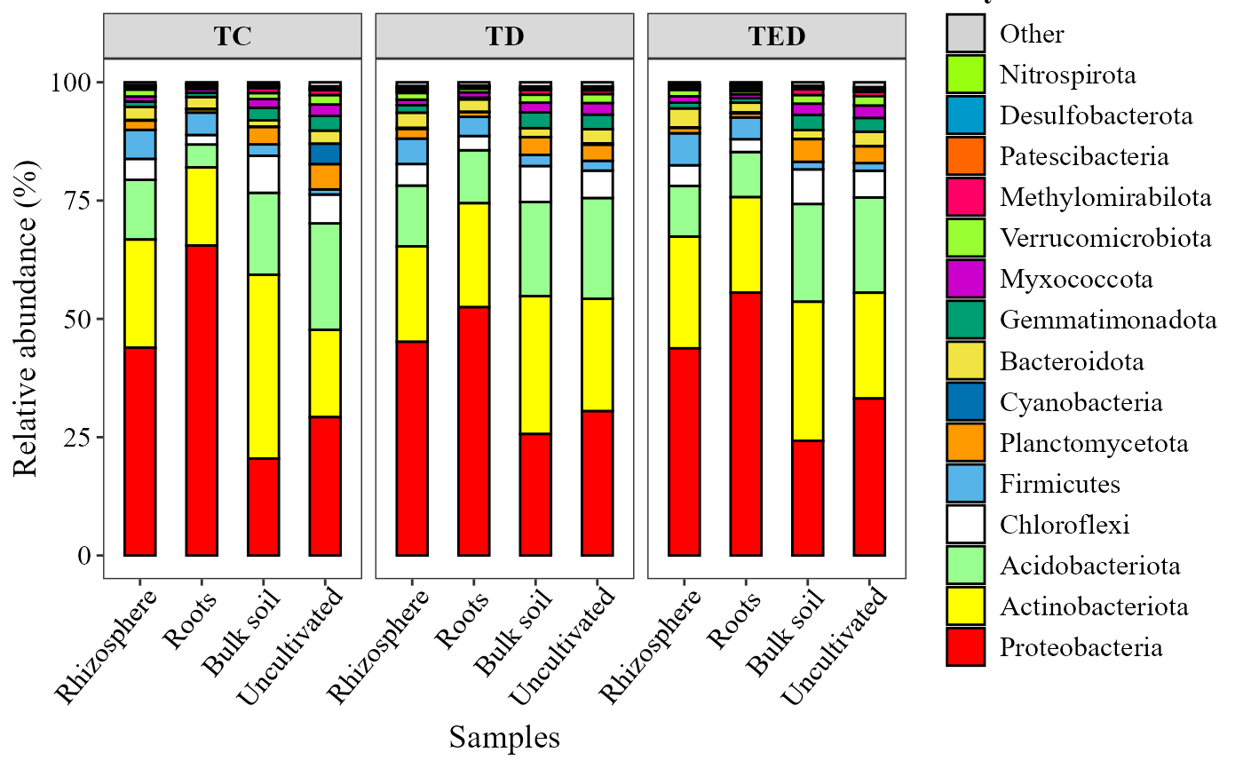
abundance_barplot(table = table_fung,
                  metadata = metadata_fungi,
                  x_col = "Treatment",
                  facet_col = "Type_of_soil",
                  add_remained = TRUE,
                  label =   "Genera",
                  save_table = FALSE)+
  theme(axis.text.x = element_text(angle = 50, hjust = 0.95))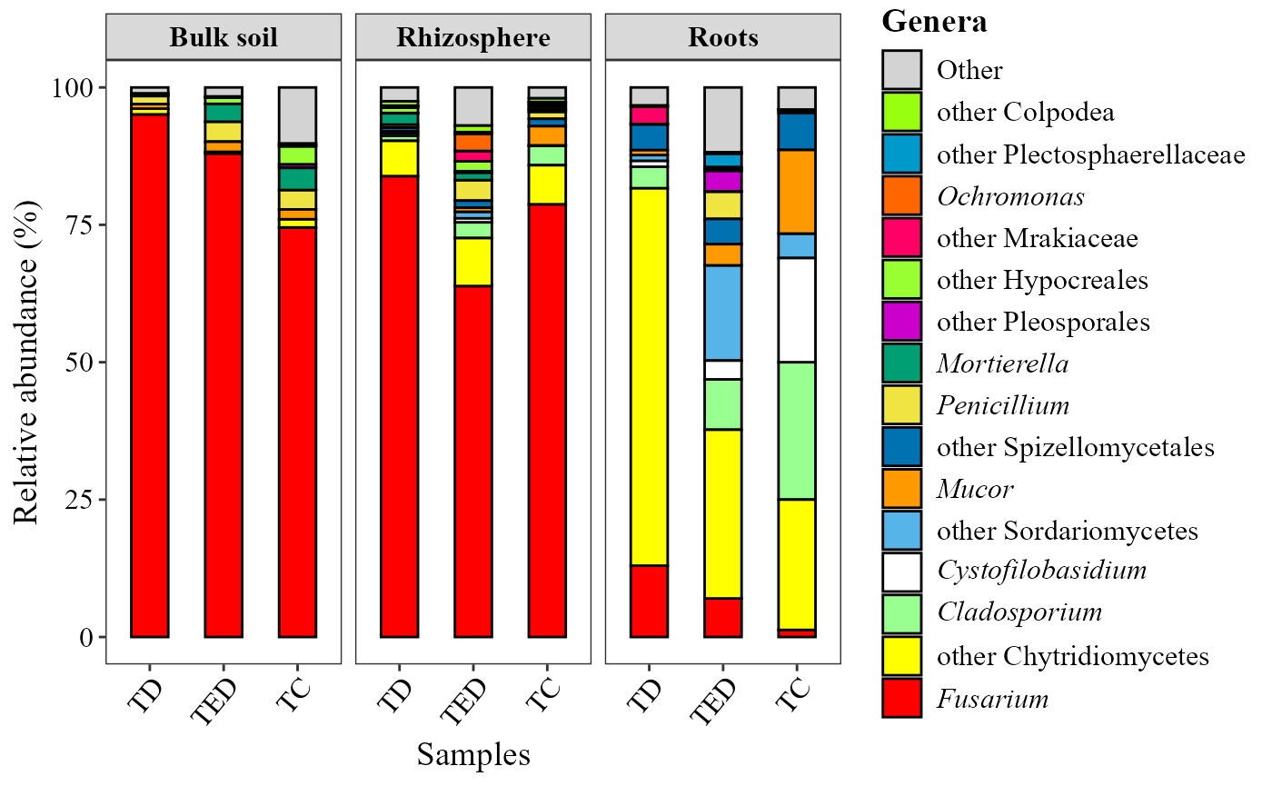
Abundance heatmaps
The input table must be a data frame containing
taxonomic features (rows) and samples (columns).
The metadata argument provides sample-level information
used to annotate the heatmap.
The parameters condition1, condition2, and
condition3 define up to three metadata variables to be
displayed as horizontal annotations above the heatmap.
Custom color palettes for each annotation can be specified using
colors_condition1, colors_condition2, and
colors_condition3, respectively.
Legend titles for these annotations can be customized with
name_legend_condition1,
name_legend_condition2, and
name_legend_condition3.
The top_n argument controls the number of most abundant
features included in the heatmap.
If cluster = TRUE, rows are hierarchically clustered; if
FALSE, features are ordered by decreasing relative
abundance.
The show_column_names parameter determines whether sample
names are displayed in the heatmap.
abundance_heatmap_plot(table = table_bac,
                  metadata = metadata_bacteria,
                  top_n = 30,
                  show_column_names = FALSE,
                  condition1 = "Type_of_soil",
                  condition2 = "Treatment")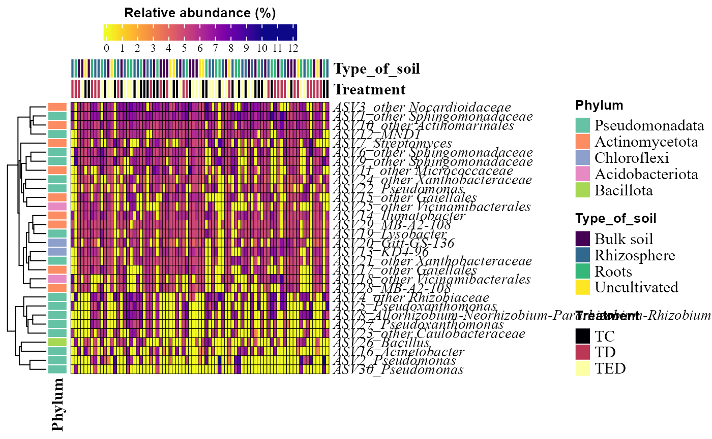
abundance_heatmap_plot(table = table_fung,
                  metadata = metadata_fungi,
                  top_n = 30,
                  show_column_names = FALSE,
                  condition1 = "Type_of_soil",
                  condition2 = "Treatment")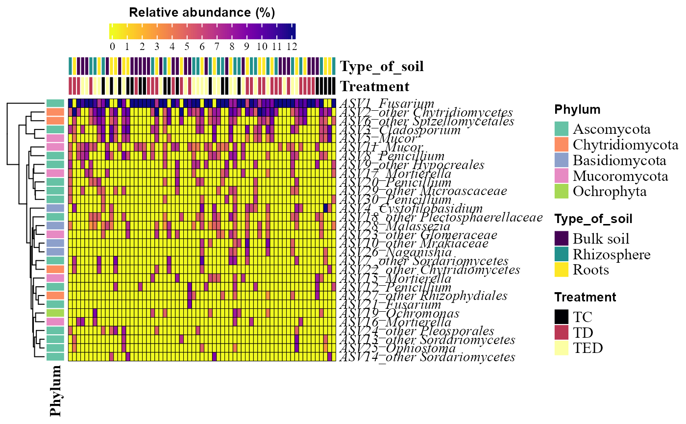
Alpha diversity
Alpha diversity describes the diversity within individual samples. In
MicroBioMeta, alpha diversity can be explored using several
metrics, including traditional indices such as richness, Shannon, and
Simpson. In addition, the package implements functions based on the
Hill numbers framework, which provides a unified way to
represent these indices as members of the same family of diversity
measures. Hill numbers are parameterized by the order q, which
controls the sensitivity of the metric to species abundances. For
example, q=0 corresponds to species richness, q=1 to
the exponential of Shannon entropy, and q=2 to the inverse
Simpson index. This formulation facilitates consistent comparison among
diversity measures and allows researchers to evaluate how diversity
patterns change depending on the weight given to rare versus abundant
taxa.
Correlation among Hill numbers
The alpha_hill_corrplot() function calculates Hill
numbers for different orders (typically, 𝑞=0,1,2) and visualizes the
correlations among them using a correlation plot.
This plot helps evaluate how strongly diversity metrics of different orders are related to the depth sequencing.
The table argument must be a data frame containing features (rows) and samples (columns).
For the bacteria, we can observed that at all orders of q there is a strong correlation with sequencing depth.
alpha_hill_corrplot(table = table_bac)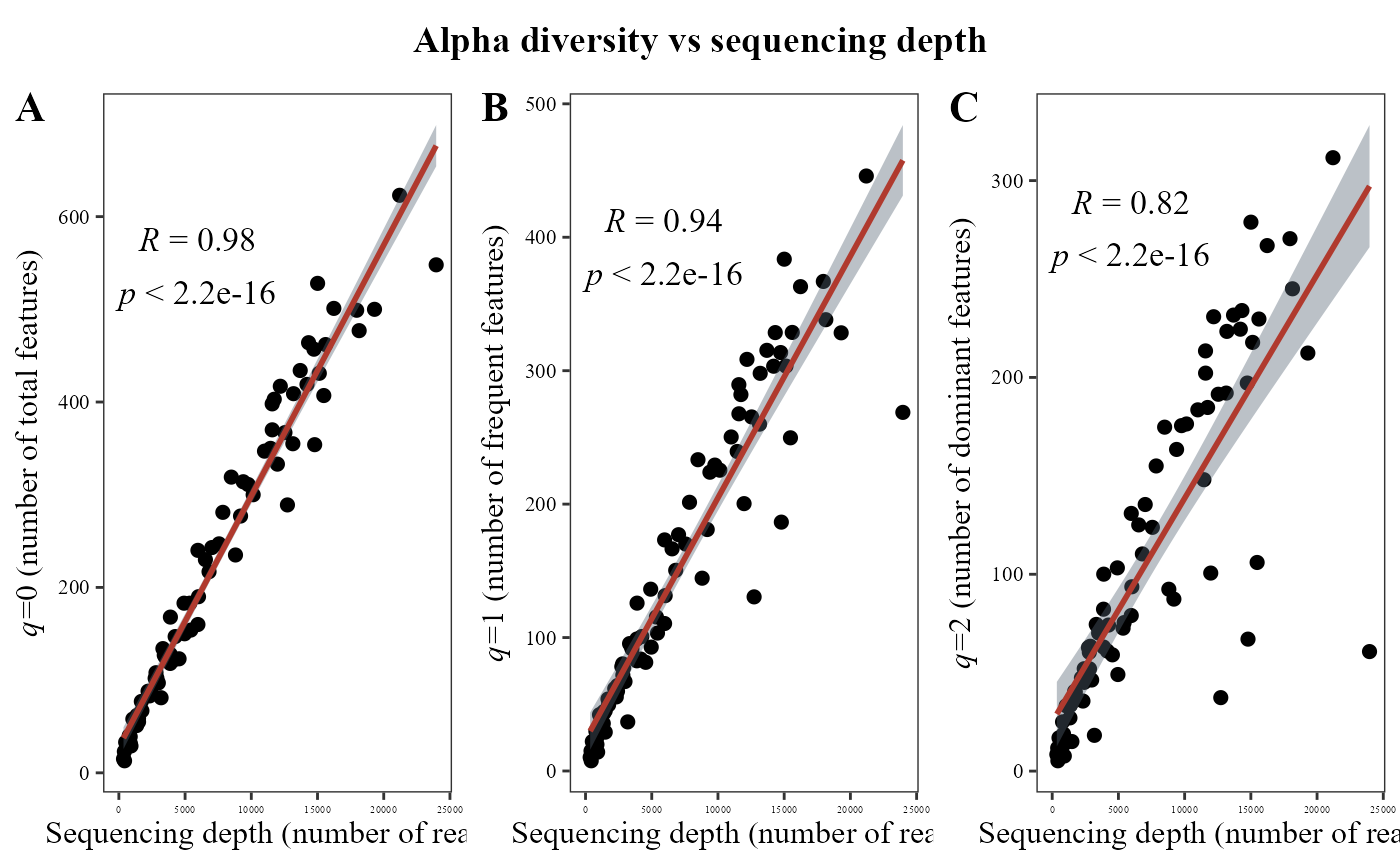
But, for fungi data this correlation is just strong and significative at q=0, it means for richness but not to the others q orders.
alpha_hill_corrplot(table = table_fung)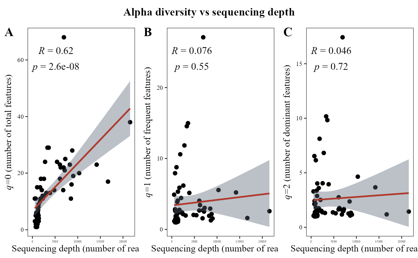
Alpha diversity visualization
The alpha_hill_plot() function calculates Hill numbers
and visualizes alpha diversity patterns across experimental conditions
using boxplots.
The metadata argument provides sample-level information
used to group and visualize the samples.
The x_col parameter specifies the metadata column used
on the x-axis, while fill_col controls the grouping used to
color the boxplots.
The facet_by argument allows splitting the plot
according to a metadata variable, and facet_orientation
controls whether facets are arranged horizontally or vertically.
If save_table = TRUE, the function also returns a table
containing the alpha diversity values calculated for each sample.
alpha_hill_plot(table = table_bac,
                metadata = metadata_bacteria,
                x_col = "Treatment",
                fill_col = "Treatment",
                facet_by = "Type_of_soil",
                facet_orientation = "vertical",
                save_table = FALSE)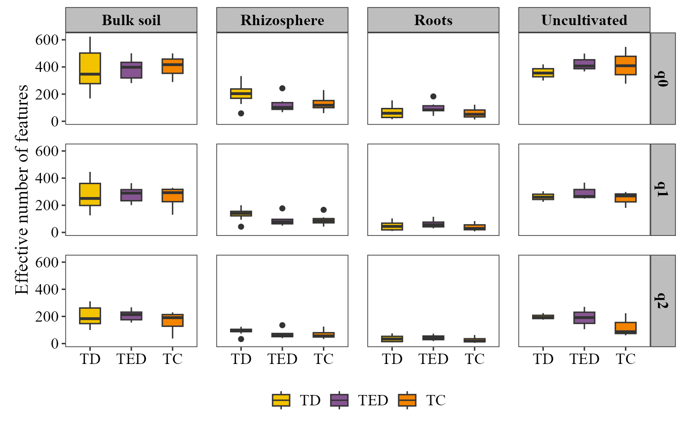
alpha_hill_plot(table = table_fung,
                metadata = metadata_fungi,
                x_col = "Treatment",
                fill_col = "Treatment",
                facet_by = "Type_of_soil",
                facet_orientation = "horizontal",
                save_table = FALSE)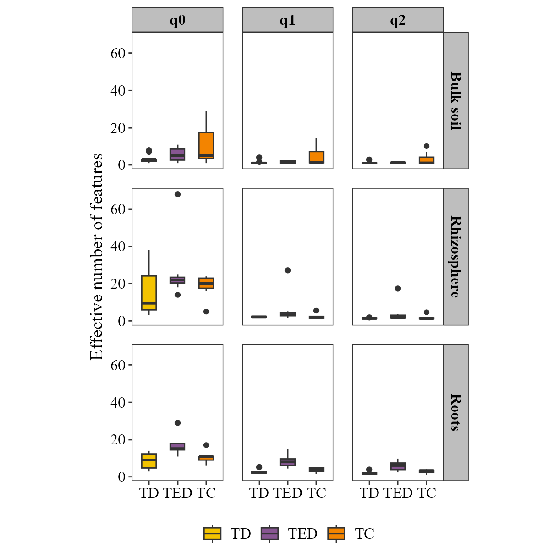
Also, we can visualize other metrics considering classic alpha diversity indexes. Also, using the parameter stat it is possible to set an statistical comparison indication the method to use:
alpha_diversity_plot(table = table_fung,
                metadata = metadata_fungi,
                x_col = "Treatment",
                fill_col = "Treatment",
                facet_by = "Type_of_soil",
                facet_orientation = "horizontal",stat = "anova",
                save_table = FALSE)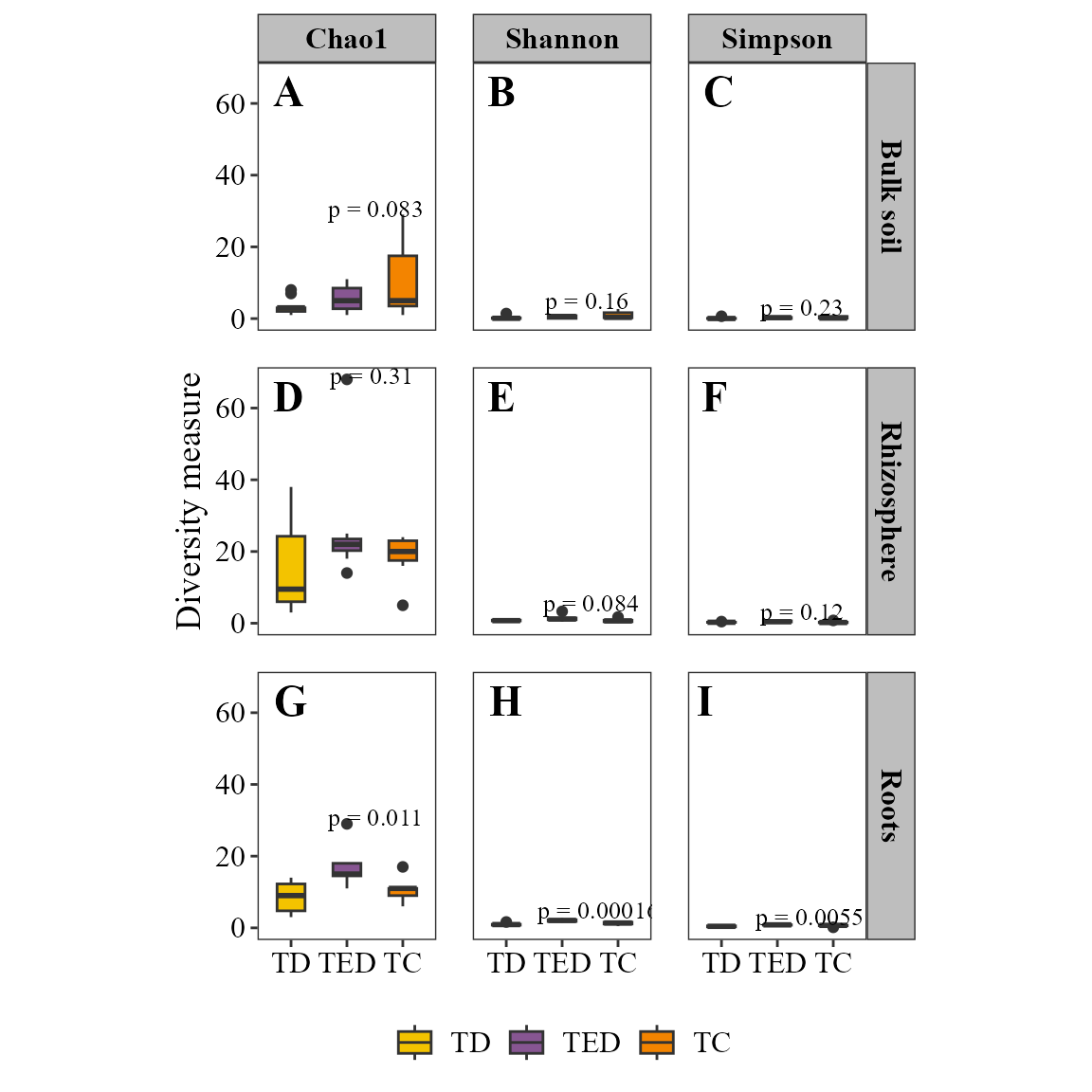
Shared taxa between sample groups
Another way to explore alpha diversity patterns is by examining
which taxa are shared or unique among groups of
samples. The function venn_diagram_plot()
generates Venn diagrams that summarize the overlap of taxa between
groups defined in the metadata.
The function can optionally filter taxa using a minimum prevalence threshold, allowing the visualization to focus only on taxa consistently detected within each group.
Next, we generate a Venn diagram grouping samples according to the soil compartment.
venn_diagram_plot(table = table_fung,
                  metadata = metadata_fungi,
                  merge_by = "Type_of_soil",
                  min_prevalence = 0 )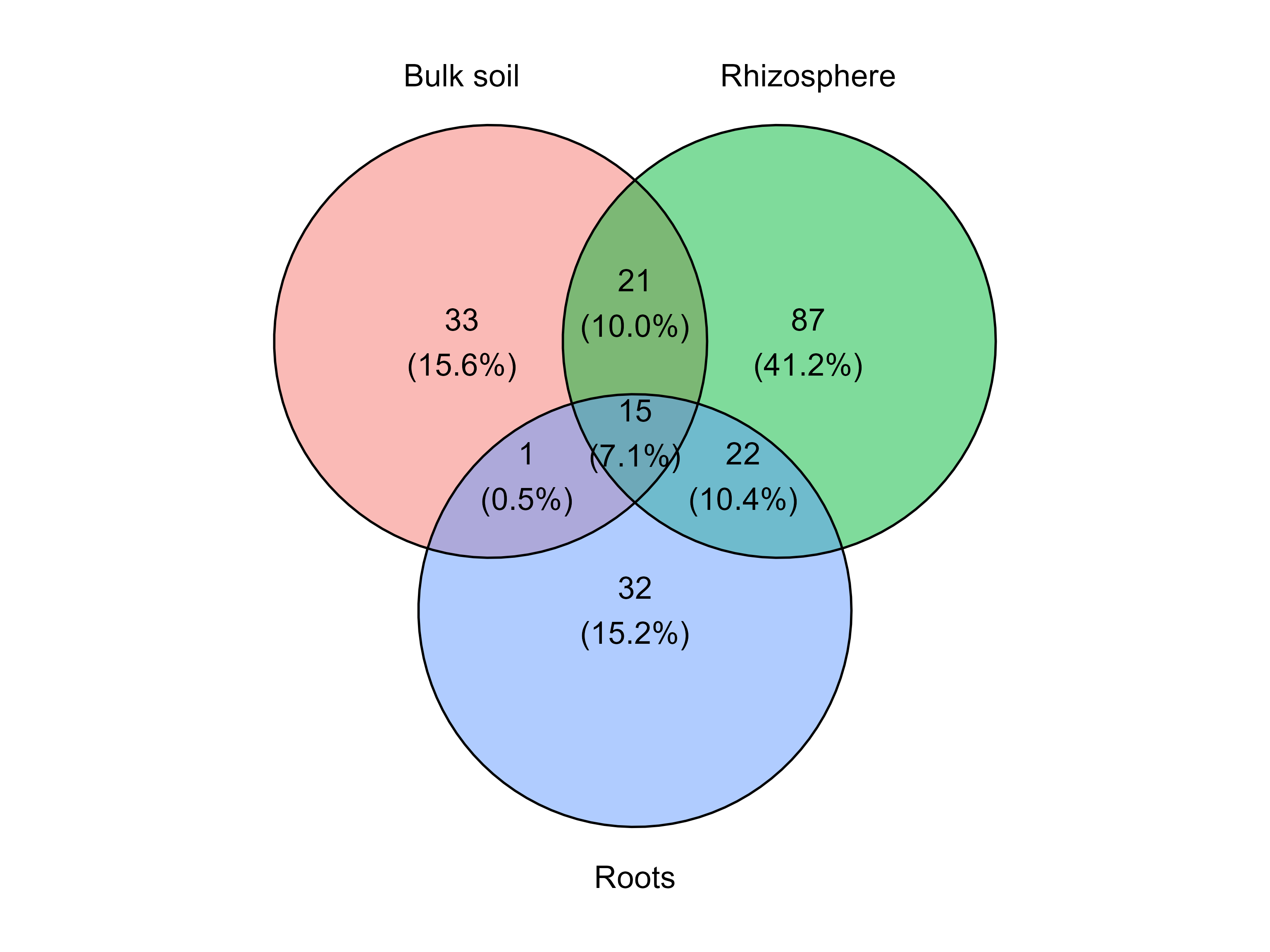
This plot shows the number of taxa that are unique to each soil compartment and those shared among groups.
Collapsing the table by taxonomic level
Microbial community tables are often generated at the ASV or OTU level, which can contain hundreds or thousands of features. For interpretation and visualization, it is often useful to aggregate these features at a higher taxonomic rank, such as genus or family.
The function collapse_table() performs this aggregation
by grouping features that share the same taxonomy at a specified level
and summing their abundances across samples. Taxa that do not reach the
selected taxonomic resolution are retained without modification.
The function returns a list with two elements:
collapsed_table: a wide-format abundance table where rows correspond to taxa collapsed at the selected level and columns correspond to samples.long_format: the same information in long format, which is useful for downstream plotting or statistical analyses.For example, the following code collapses the fungal abundance table to the genus level.
table_genus <- collapse_table(
  table = table_fung,
  metadata = metadata_fungi,
  level = "genus"
)

venn_diagram_plot(
  table = table_genus$collapsed_table,
  metadata = metadata_fungi,
  merge_by = "Type_of_soil"
)
By default, collapse_table() returns the raw
counts summed at the selected taxonomic level. However,
microbial community data are often easier to interpret when expressed as
relative abundance, since sequencing depth can vary
across samples.
Setting rel_abun = TRUE converts the counts of each
sample into percentages, where the total abundance per
sample sums to 100%.
Filtering taxa by prevalence
Sometimes it is useful to visualize only taxa that occur frequently
within each group. This can be done using the
min_prevalence parameter.
For example, the following diagram includes only taxa present in at least 20% of the samples within each group.
venn_diagram_plot(table = table_fung,
                  metadata = metadata_fungi,
                  merge_by = "Type_of_soil",
                  min_prevalence = 0.2 )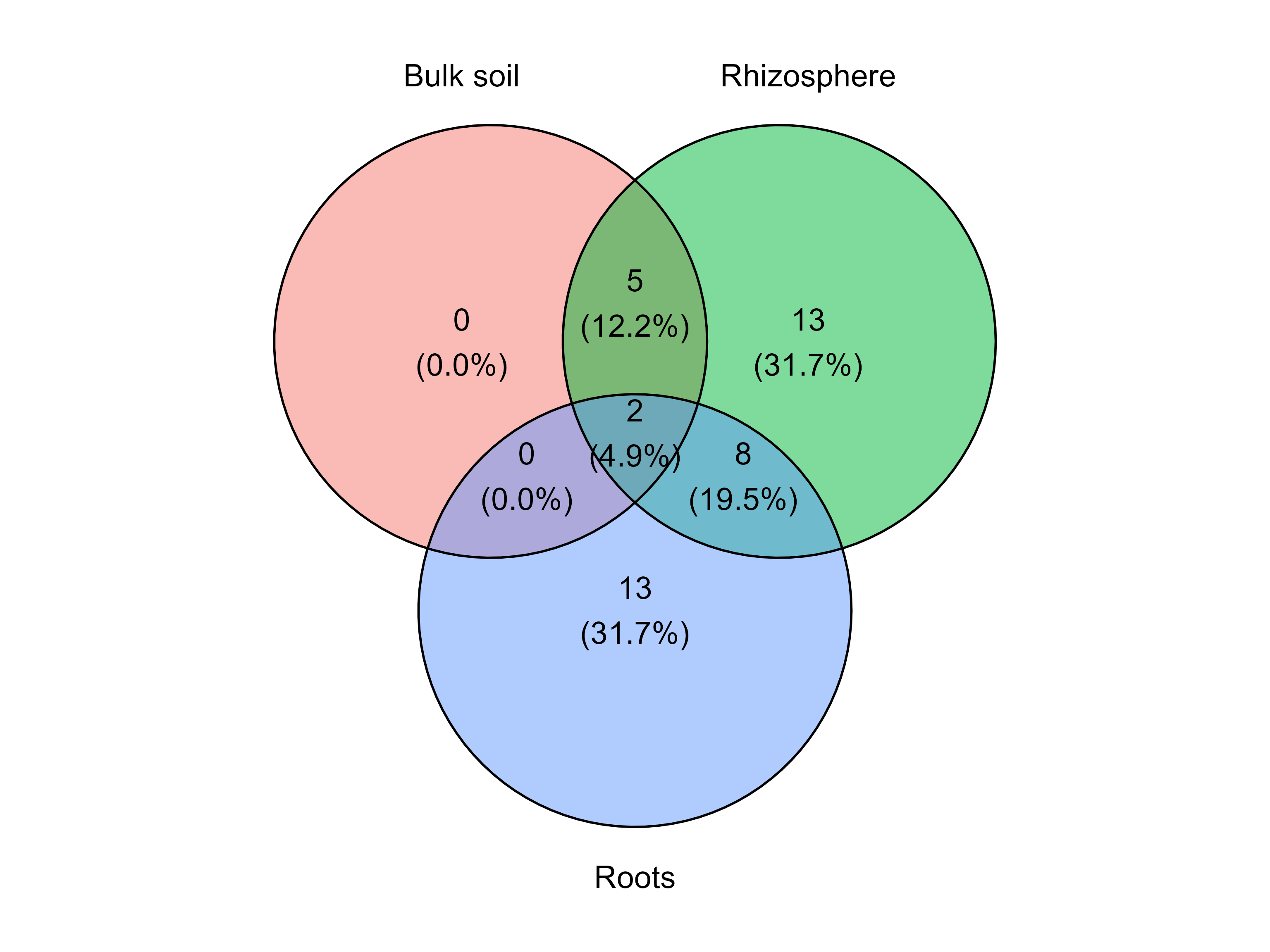
Customizing group colors
The function also allows custom colors for the groups.
venn_diagram_plot(table = table_fung,
                  metadata = metadata_fungi,
                  merge_by = "Type_of_soil",
                  min_prevalence = 0,
                  group_colors = c("#1B9E77", "#D95F02", "#7570B3") )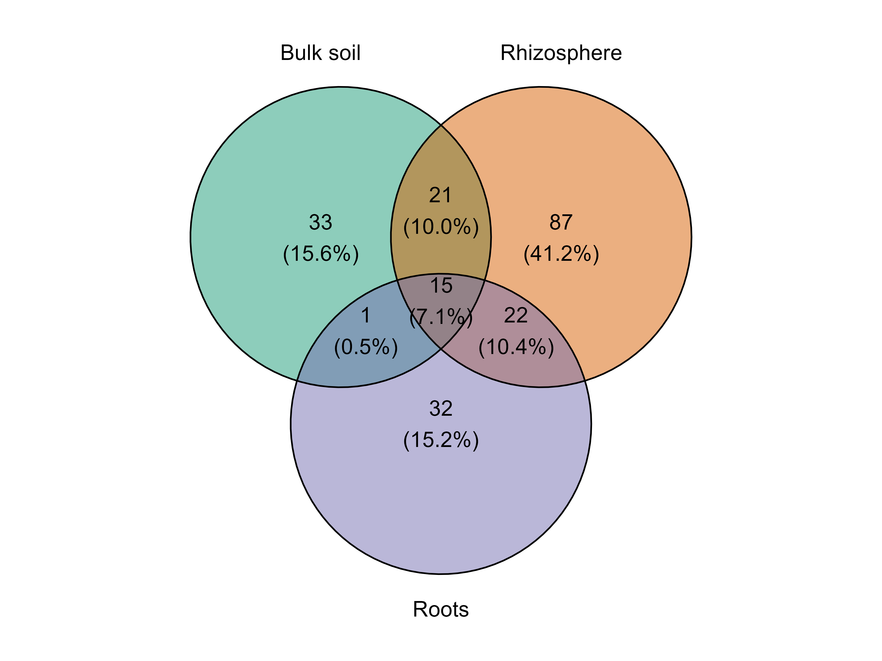
Alternative plotting method
By default the function uses the package ggvenn, but it can also generate the diagram using ggVennDiagram.
venn_diagram_plot(table = table_fung,
                  metadata = metadata_fungi,
                  merge_by = "Type_of_soil",
                  method = "ggvenndiagram" )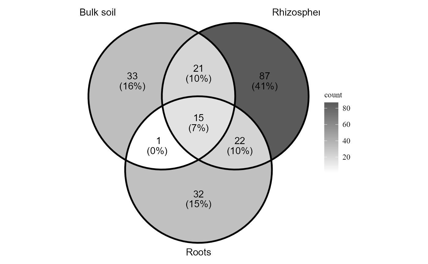
Beta diversity
Beta diversity describes the differences in community composition among samples. These analyses help determine whether microbial communities vary across environmental conditions, treatments, or experimental groups.
MicroBioMeta provides several tools to explore beta
diversity, including ordination methods, statistical tests for community
differences, and partitioning approaches that separate shared and unique
components of diversity. These functions allow both visual exploration
of compositional patterns and formal hypothesis testing.
Ordination of community composition
The beta_div_plot() function calculates pairwise
dissimilarities among samples and visualizes the results using an
ordination method. By default, the function uses common ecological
distance metrics (e.g., Bray–Curtis or Euclidean) and dimensionality
reduction techniques such as PCoA,
PCA, or NMDS. Accounting for
compositional data in the examples aitchinson and
compositional distances are used. Compositional refers to
the clr (log centered ratio) transformation made by
ALDEx2 package.
The group_col parameter specifies the metadata column
used to color the samples, while shape_col allows an
additional metadata variable to be displayed using different point
shapes.
The distance argument defines the dissimilarity metric
used to calculate beta diversity, and ordination specifies
the ordination method applied to visualize the distances among
samples.
beta_div_plot(table = table_bac,
              metadata = metadata_bacteria,
               distance = "compositional",
              ordination = "PCA",
              group_col = "Type_of_soil",
              shape_col = "Treatment")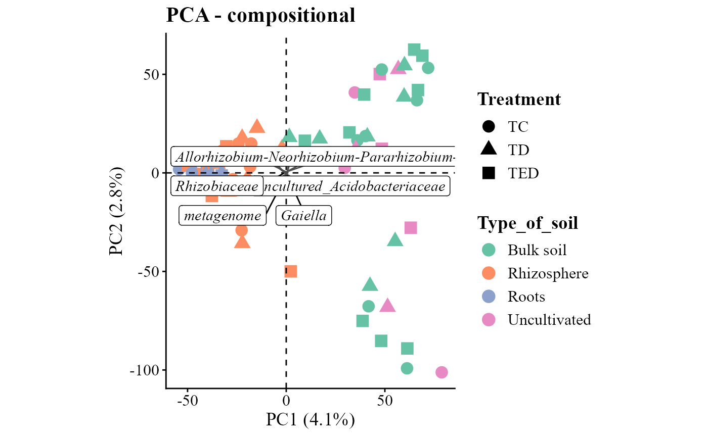
beta_div_plot(table = table_fung,
              metadata = metadata_fungi,
              group_col = "Type_of_soil",
              shape_col = "Treatment",
              distance = "aitchison",
              ordination = "NMDS")
## Run 0 stress 0.1631777
## Run 1 stress 0.1761678
## Run 2 stress 0.1711358
## Run 3 stress 0.1794788
## Run 4 stress 0.1807005
## Run 5 stress 0.1684556
## Run 6 stress 0.1780017
## Run 7 stress 0.1774533
## Run 8 stress 0.1780714
## Run 9 stress 0.1694127
## Run 10 stress 0.1727115
## Run 11 stress 0.1738753
## Run 12 stress 0.1669527
## Run 13 stress 0.1718431
## Run 14 stress 0.1630755
## ... New best solution
## ... Procrustes: rmse 0.09922073 max resid 0.665334
## Run 15 stress 0.1809031
## Run 16 stress 0.1784415
## Run 17 stress 0.1725226
## Run 18 stress 0.1679461
## Run 19 stress 0.1729715
## Run 20 stress 0.1751556
## Run 21 stress 0.1773671
## Run 22 stress 0.1763503
## Run 23 stress 0.1798722
## Run 24 stress 0.1753608
## Run 25 stress 0.1714175
## Run 26 stress 0.1751582
## Run 27 stress 0.1754506
## Run 28 stress 0.1710514
## Run 29 stress 0.1663737
## Run 30 stress 0.1630904
## ... Procrustes: rmse 0.001130218 max resid 0.005048388
## ... Similar to previous best
## *** Best solution repeated 1 times## Coordinate system already present.
## ℹ Adding new coordinate system, which will replace the existing one.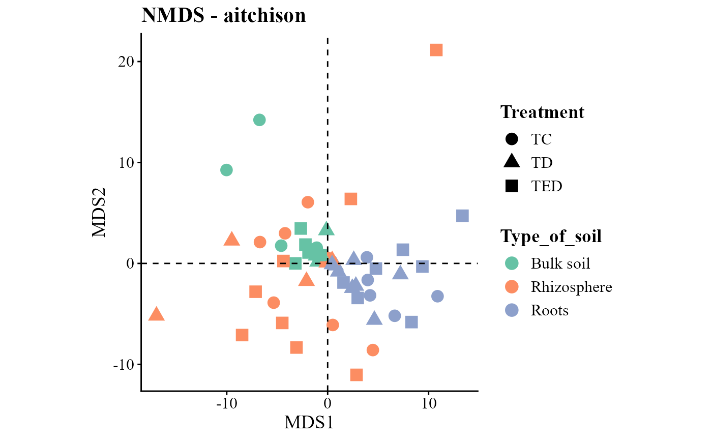
Statistical tests for beta diversity
The beta_test_table() function performs statistical
tests to evaluate whether community composition differs among
experimental groups.
The formula_str argument specifies the experimental
design using a formula syntax similar to linear models in R. The
method parameter defines the distance metric used to
calculate dissimilarities, and the test argument specifies
the statistical method (e.g., PERMANOVA).
The permutations parameter determines the number of
permutations used to estimate statistical significance.
beta_test_table(table = table_bac,
                metadata= metadata_bacteria,
                formula_str = "Type_of_soil*Treatment",
                method = "euclidean",
                test = "permanova",
                permutations = 999)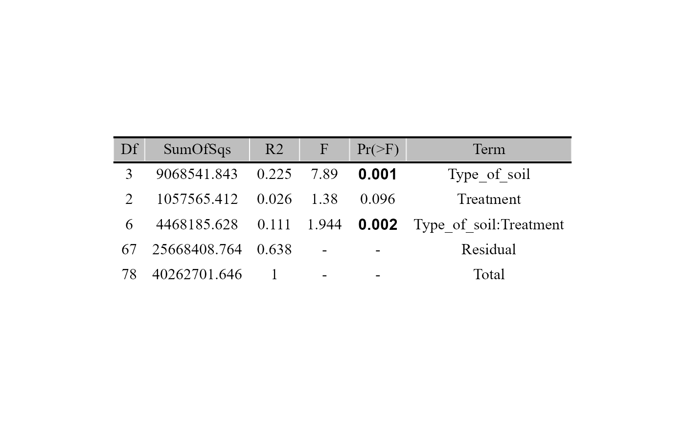
beta_test_table(table = table_fung,
                metadata= metadata_fungi,
                formula_str = "Type_of_soil*Treatment",
                method = "euclidean",
                test = "permanova",
                permutations = 999)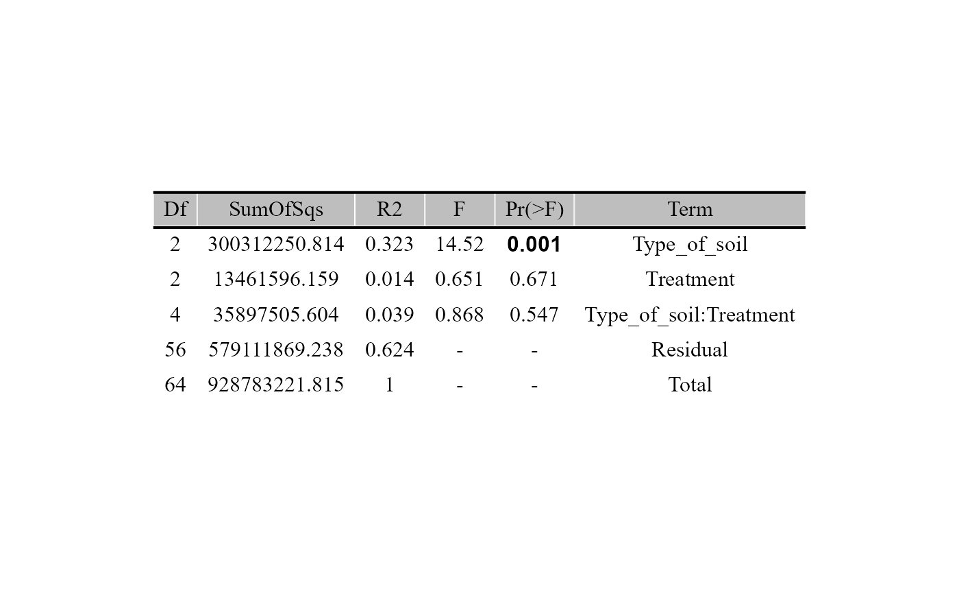
Beta diversity partitioning
Beta diversity can also be decomposed into different components that
describe how communities differ. The beta_partition_plot()
function partitions beta diversity into shared and unique fractions
based on selected dissimilarity indices.
The index argument specifies the dissimilarity family
used for the partition (e.g., Jaccard or Sørensen). The
group_col and shape_col parameters define how
samples are visualized according to metadata variables.
beta_partition_plot(
  table = table_bac,
  metadata = metadata_bacteria,
  index = "jaccard",
  group_col = "Type_of_soil",
  shape_col = "Treatment",
  save_table = FALSE)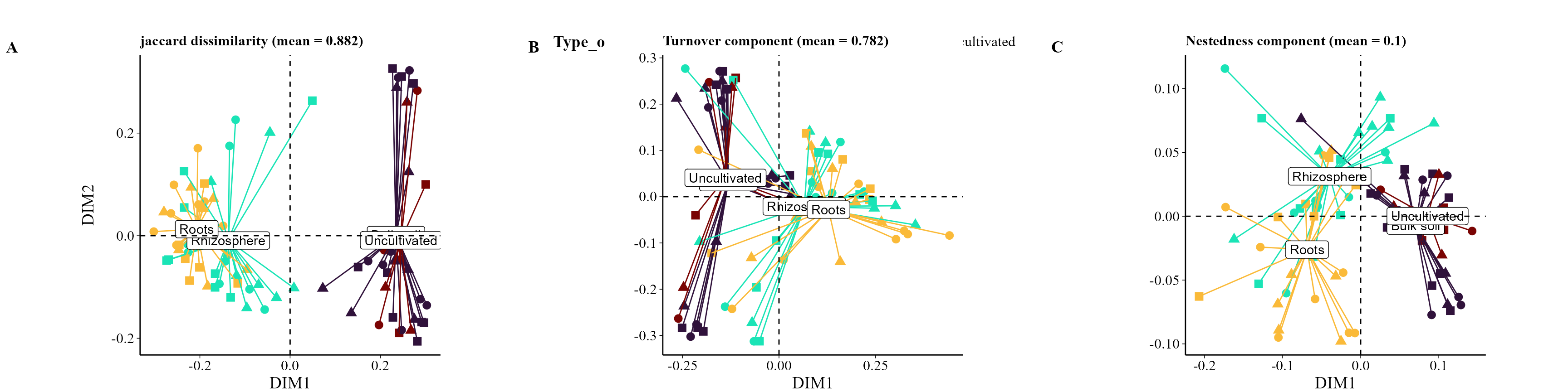
beta_partition_plot(
  table = table_fung,
  metadata = metadata_fungi,
  index = "jaccard",
  group_col = "Type_of_soil",
  shape_col = "Treatment",
  save_table = FALSE)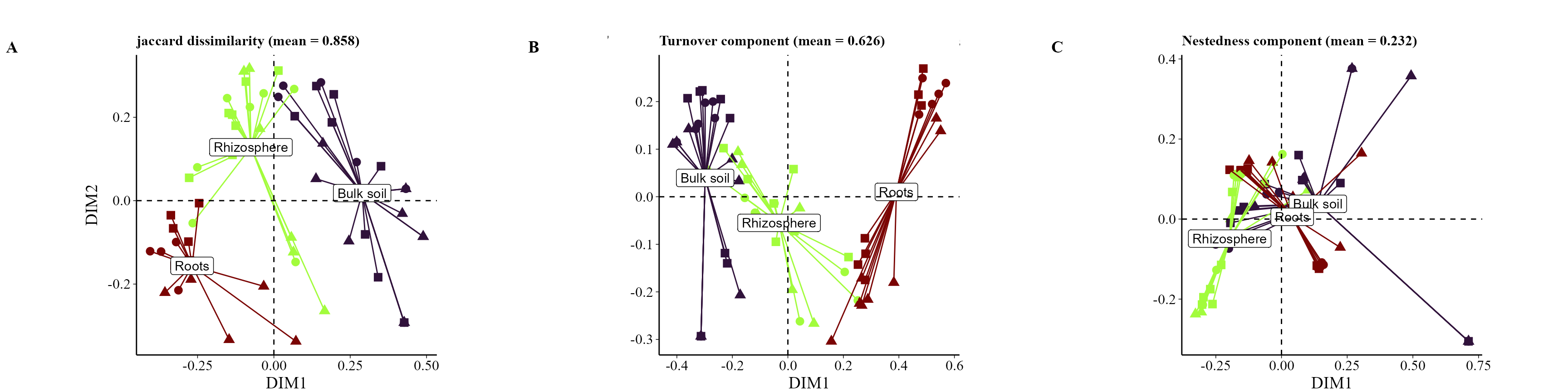
Pairwise beta diversity visualization
The beta_diversity_boxplot() function summarizes
pairwise beta diversity values using boxplots, allowing comparison of
diversity patterns among groups of samples.
The condition1_col and condition2_col
parameters specify metadata variables used to define the groups being
compared. The partition argument determines which component
of beta diversity is displayed (e.g., shared or unique), while
family defines the dissimilarity index used.
If save_table = TRUE, the function also returns a table
containing the beta diversity values used to generate the plot.
beta_diversity_boxplot(table = table_bac,
                       metadata = metadata_bacteria,
                       condition1_col = "Type_of_soil",
                       condition2_col = "Treatment",
                       title_axis_x = "Samples",
                       partition = "shared", family = "jaccard",
                       save_table = FALSE)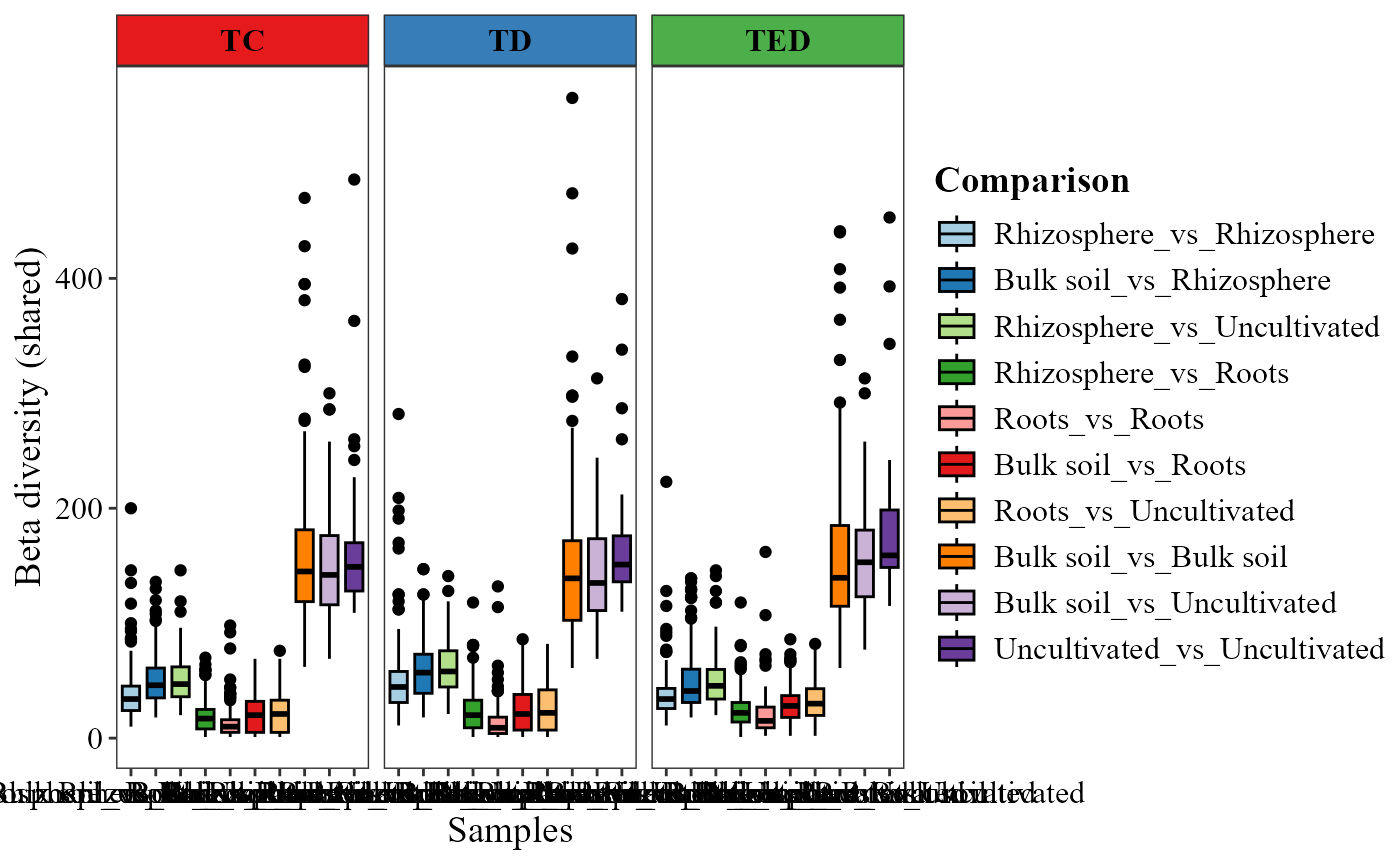
beta_diversity_boxplot(table = table_fung,
                       metadata = metadata_fungi,
                       condition1_col = "Type_of_soil",
                       condition2_col = "Treatment",
                       title_axis_x = "Samples",
                       partition = "shared",
                       family = "jaccard",
                       save_table = FALSE)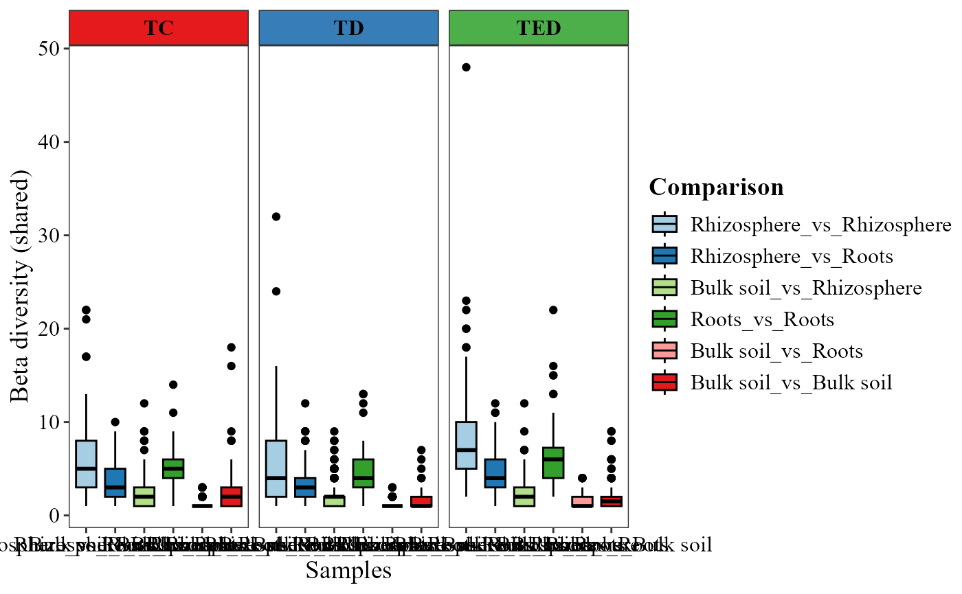
Differential abundant analysis
MicroBioMeta provides several functions to explore
differentially abundant taxa between conditions. These
analyses help identify microbial features that vary significantly across
environments or experimental groups.
Two functions rely on a compositional data analysis framework implemented in the package ALDEx2. This approach accounts for the compositional nature of sequencing data by using Monte Carlo Dirichlet instances and centered log-ratio transformations, making it more appropriate for high-throughput sequencing datasets than traditional count-based methods.
The functions:
aldex_volcano_plot()visualizes differential abundance results using a volcano plot.aldex_heatmap_plot()highlights significant taxa in a heatmap representation.Additionally, two complementary approaches help identify important taxa that discriminate between groups:
ratio_plot()highlights taxa based on log-ratio differences between conditions.randomf_lollipop_plot()uses a Random Forest model to identify features that best predict a given variable, visualized as a lollipop plot of feature importance.Since ALDEx2 performs pairwise comparisons, we first subset the data to include only two experimental conditions.
Example: Bacterial data
First, we filter the metadata to retain only two soil compartments.
metadata_bacteria_compar <-  metadata_bacteria %>%
  filter(Type_of_soil == "Roots" | Type_of_soil =="Rhizosphere")

table_bacteria_compar <- table_bacteria[match(metadata_bacteria_compar$SAMPLEID, colnames(table_bacteria))]

table_bac_compar <- merge_feature_taxonomy(table_bacteria_compar, taxonomy_bacteria)
## Warning in merge_feature_taxonomy(table_bacteria_compar, taxonomy_bacteria): 83
## taxonomy IDs are not present in the table and will be excluded from the result.We can visualize differential abundance using a volcano plot.
aldex_volcano_plot(table = table_bac_compar,
                   metadata = metadata_bacteria_compar,
                   col_cond = "Type_of_soil",
                   type = "volcano" )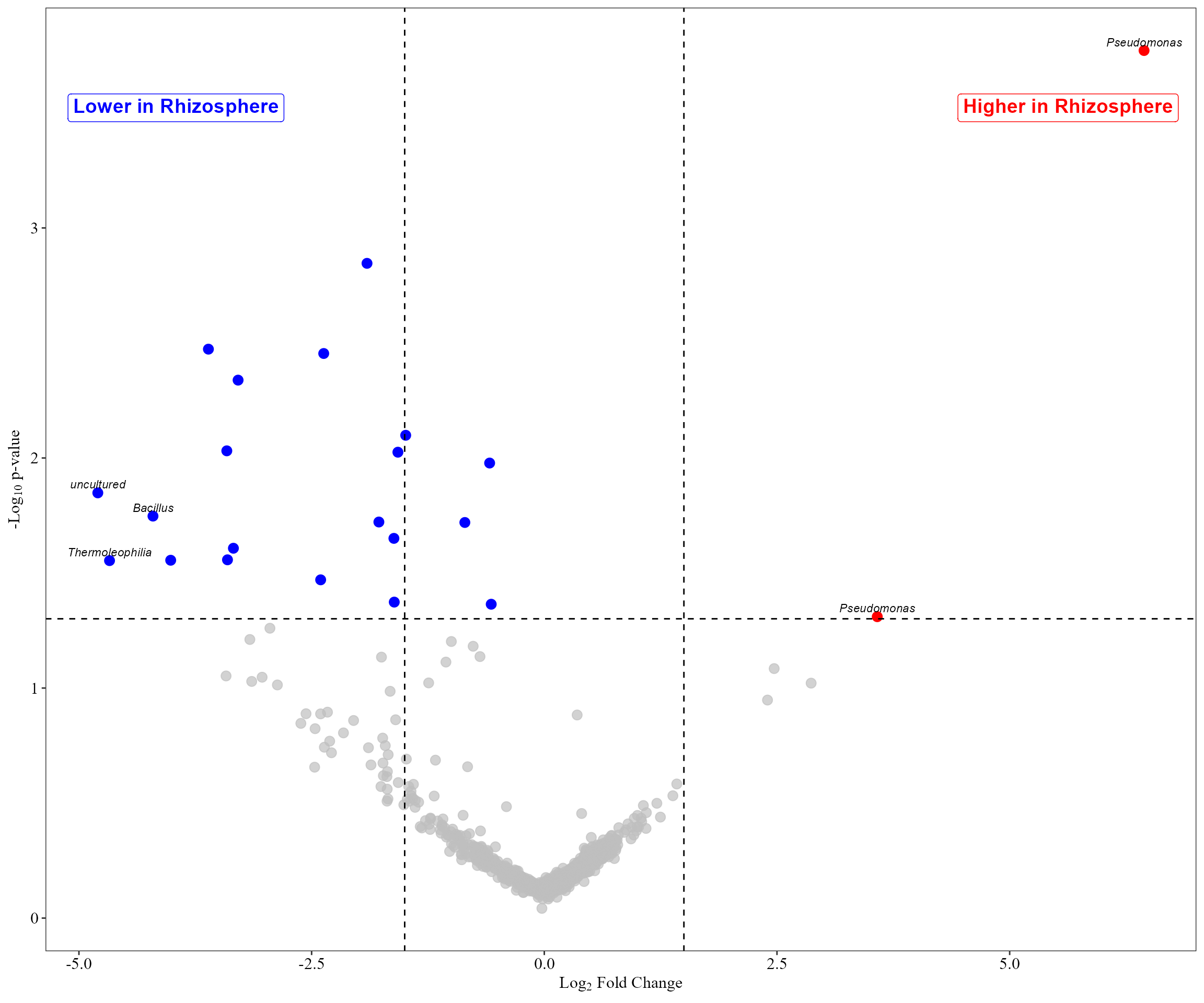
Example: Fungal data
We follow the same procedure but visualize the results with a heatmap.
metadata_fungi_compar <-  metadata_fungi %>%
  filter(Type_of_soil == "Bulk soil" | Type_of_soil =="Rhizosphere")

table_fungi_compar <- table_fung[match(metadata_fungi_compar$SAMPLEID, colnames(table_fung))]

table_fung_compar <- merge_feature_taxonomy(table_fungi_compar, taxonomy_fungi)
## Warning in merge_feature_taxonomy(table_fungi_compar, taxonomy_fungi): 17
## taxonomy IDs are not present in the table and will be excluded from the result.
aldex_heatmap_plot(table = table_fung_compar,
                   metadata = metadata_fungi_compar,
                   col_cond = "Type_of_soil")
## |------------(25%)----------(50%)----------(75%)----------|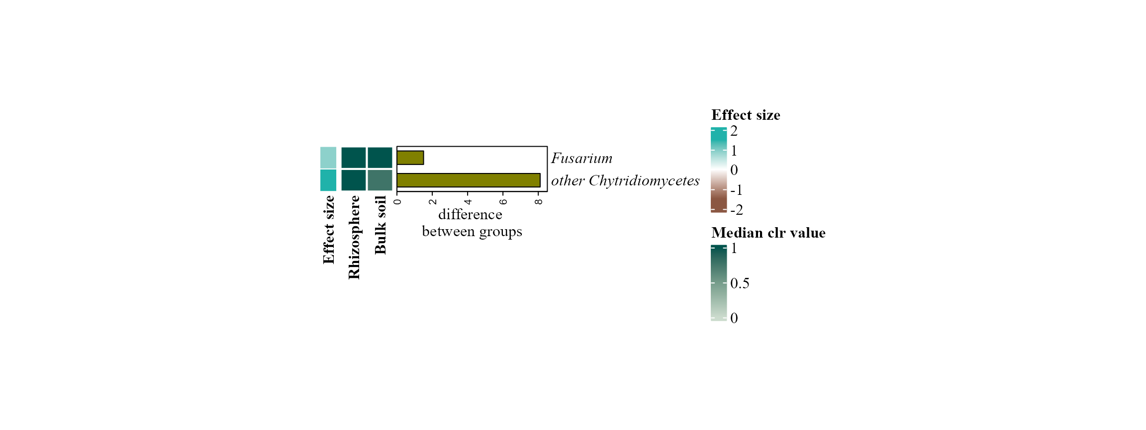
Identifying important taxa
The functions randomf_lollipop_plot() and
ratio_plot() can also be used to highlight taxa that
contribute most strongly to the observed differences between
conditions.
For example, a Random Forest model can be used to identify the taxa that best predict the soil compartment:
randomf_lollipop_plot(table = table_bac, metadata = metadata_bacteria, top_n = 10, variable_to_predict = "Type_of_soil")## Warning in randomf_lollipop_plot(table = table_bac, metadata = metadata_bacteria, : Note: Some bacterial phylum names have been updated to match NCBI's revised taxonomy:
## - 'Proteobacteria' changed to 'Pseudomonadota'
## - 'Actinobacteriota' changed to 'Actinomycetota'
## Reference: https://ncbiinsights.ncbi.nlm.nih.gov/2021/12/10/ncbi-taxonomy-prokaryote-phyla-added/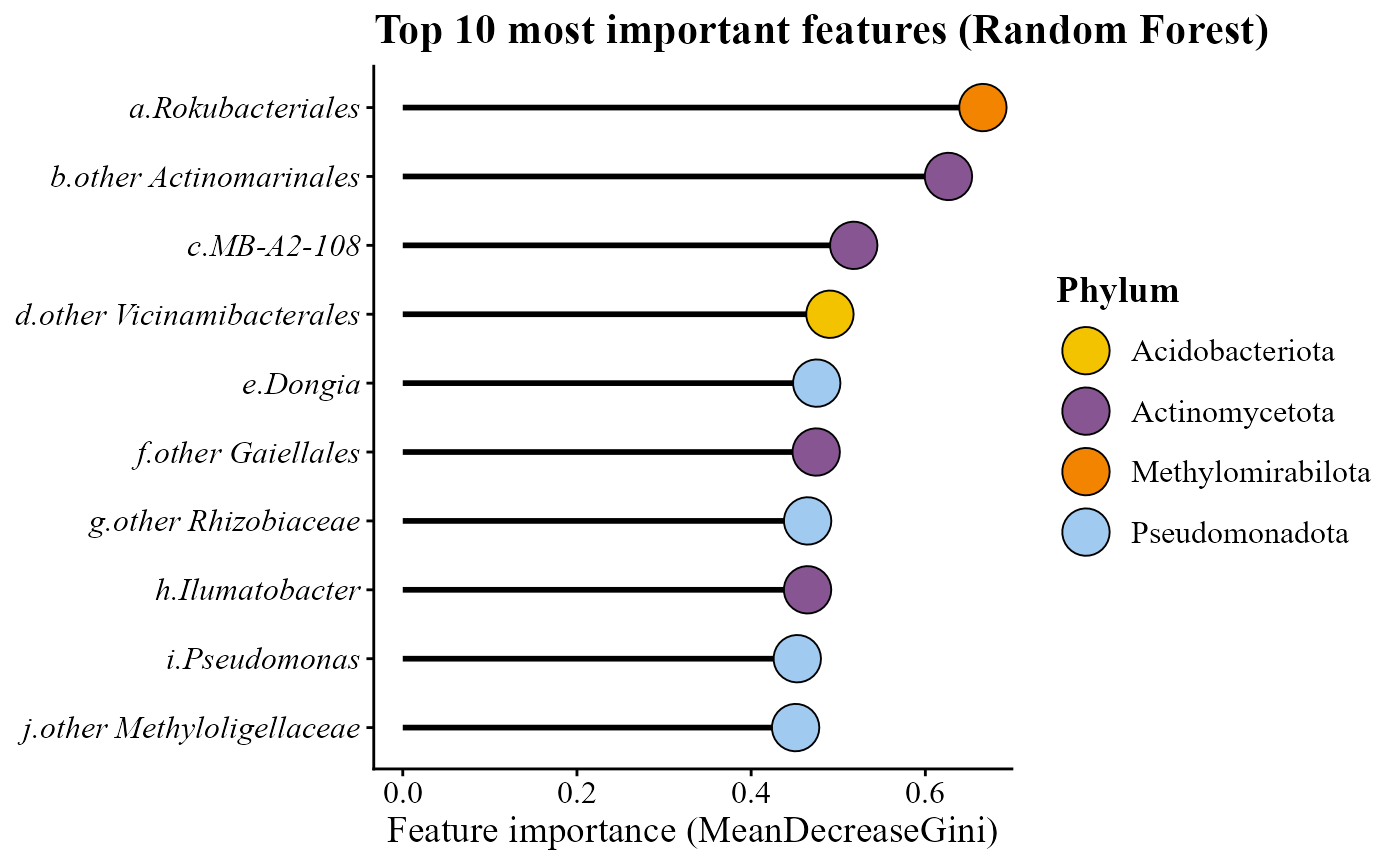
Alternatively, taxa with the strongest log-ratio differences between two conditions can be visualized using:
ratio_plot(table = table_fung_compar,
           metadata = metadata_fungi_compar,
           condition_col = "Type_of_soil",
           top_n = 20,
           condition_A = "Rhizosphere",
           condition_B = "Bulk soil")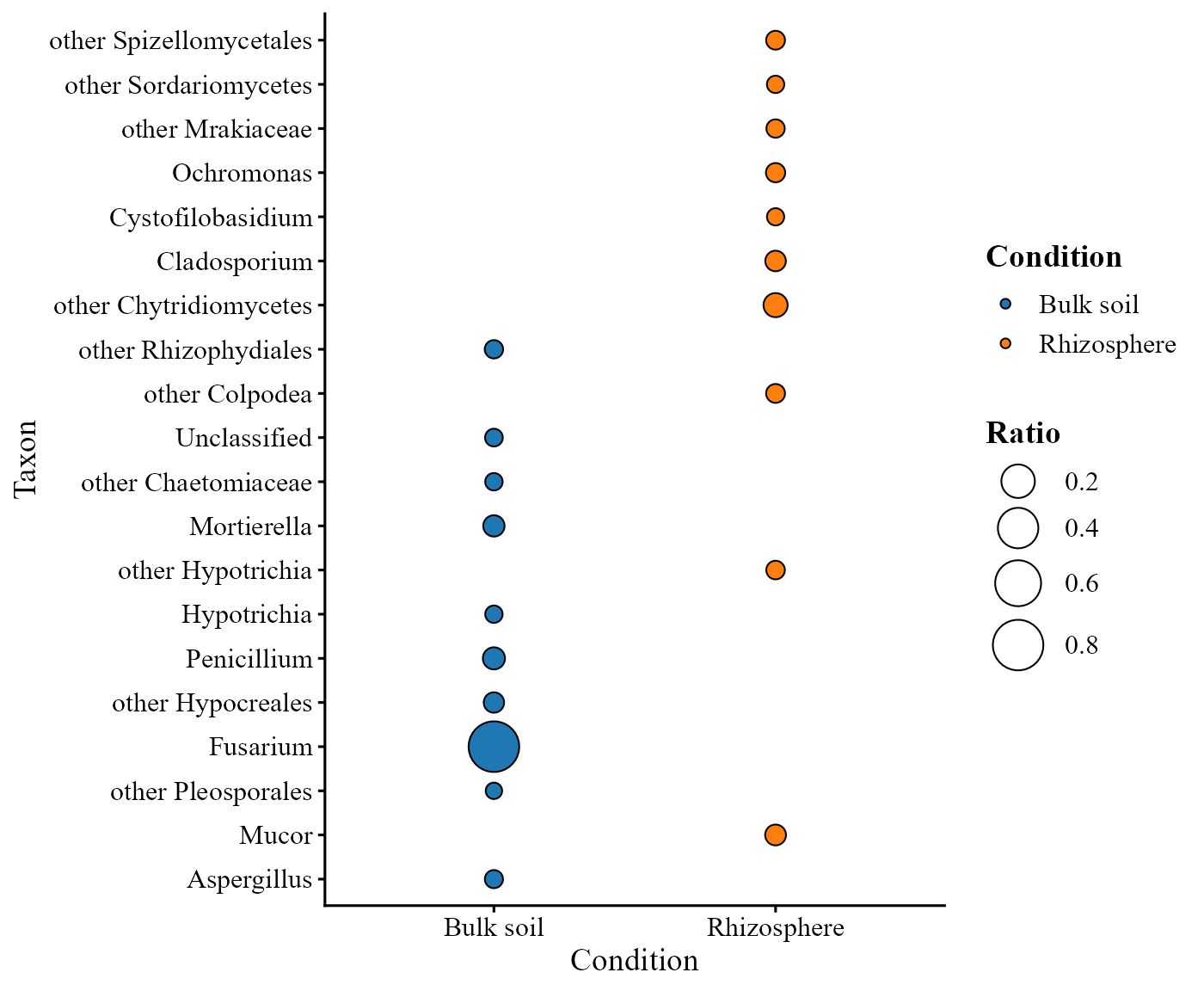
Environmental analyses
MicroBioMeta provides two functions to explore the relationship between environmental variables and microbial community composition:
corr_env_abund_plot()— computes correlations between taxonomic abundance and environmental variables.cca_rda_biplot()— performs constrained ordination using Canonical Correspondence Analysis (CCA) or Redundancy Analysis (RDA).
Preparing the environmental table
Environmental variables must be organized in a data frame where rows correspond to samples and columns correspond to environmental variables.
In this example, environmental variables are extracted from the metadata.
env_table_bac <- metadata_bacteria %>%
  dplyr::select(SAMPLEID, pH:Arbus_per) %>%
  remove_rownames() %>%
  column_to_rownames(var = "SAMPLEID")
Correlation between environmental variables and taxonomic abundance
The function corr_env_abund_plot() calculates
correlations between environmental variables and
taxonomic relative abundances at a selected taxonomic
level.
Example using phylum-level abundances:
corr_env_abund_plot(table = table_bac,
                    env_table = env_table_bac,
                    metadata = metadata_bacteria,
                    level = "phylum",
                    save_table = FALSE)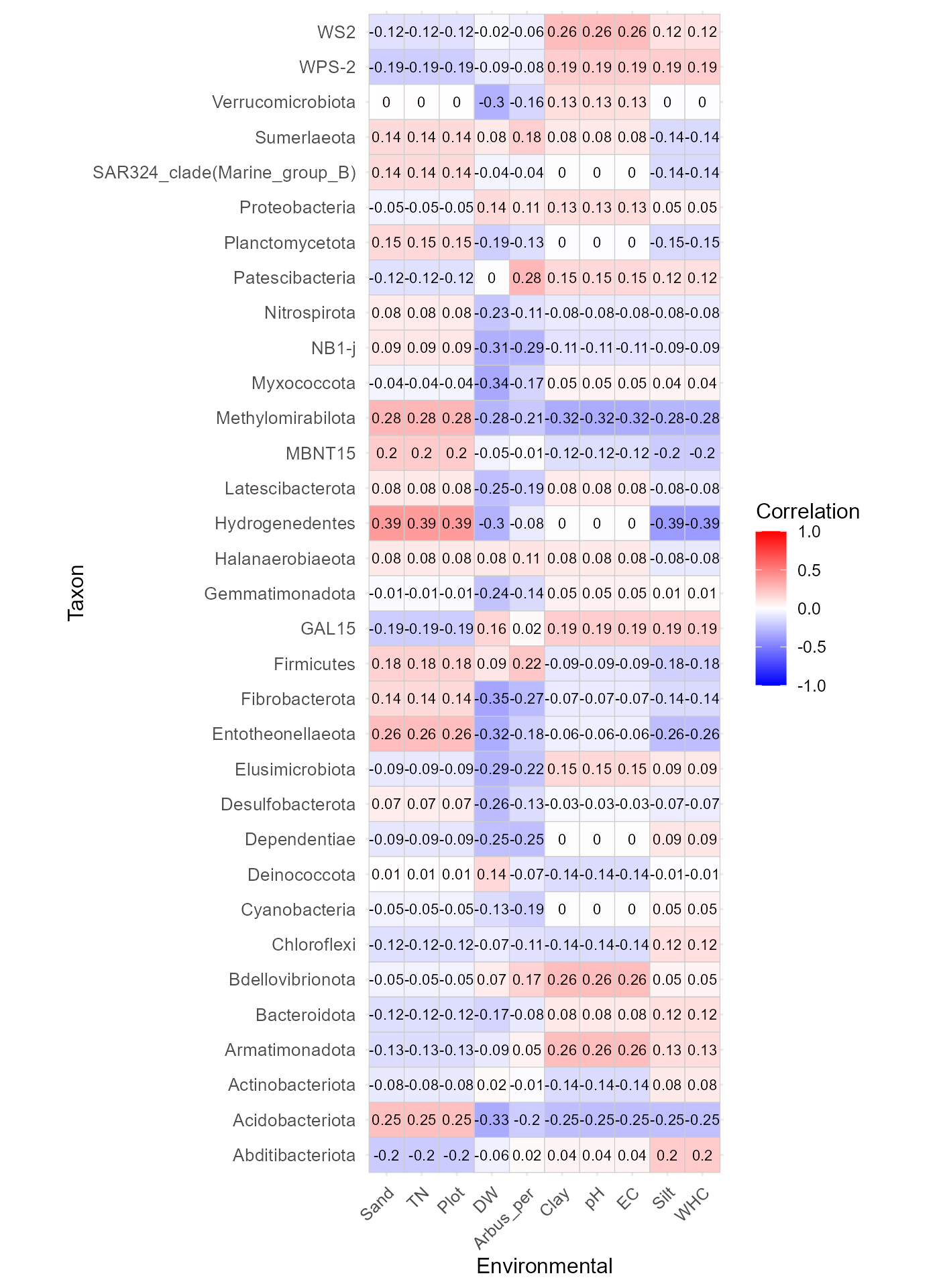
This function produces a correlation heatmap showing how environmental variables relate to taxonomic abundances.
Alternative visualization
Correlations can also be displayed using circle markers instead of tiles:
corr_env_abund_plot(table = table_bac,
                    env_table = env_table_bac,
                    metadata = metadata_bacteria,
                    level = "phylum",
                    save_table = FALSE,
                    geom = "circle")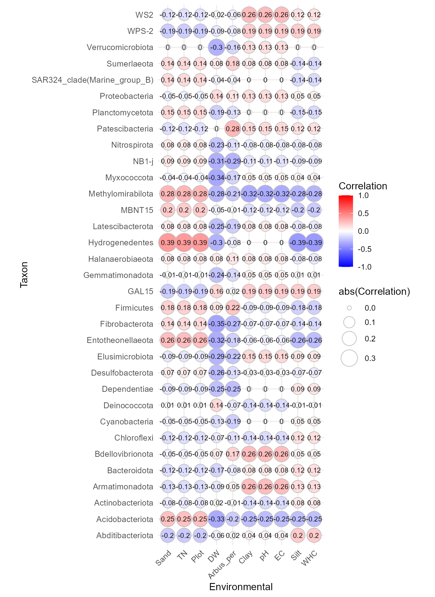
Constrained ordination (CCA / RDA)
The function cca_rda_biplot() performs a constrained
ordination analysis to evaluate how environmental variables explain
variation in microbial community composition.
Before running the analysis, ensure that the sample order in the environmental table matches the metadata.
rownames(env_table_bac) <- env_table_bac$SAMPLEID

env_table_bac <- env_table_bac[
  match(metadata_bacteria$SAMPLEID, rownames(env_table_bac)), ]
Then run the RDA analysis:
cca_rda_biplot(table = table_bac,
               env_data = env_table_bac,
               metadata = metadata_bacteria,
               env_vars = c("pH","TN","WHC", "EC", "Clay"),
               analysis = "RDA",
               show_all_env_vectors = TRUE,
               group_col = "Type_of_soil")
This analysis produces a biplot where:
Points represent samples
Colors indicate sample groups defined in the metadata.
Arrows represent environmental variables and their direction of influence on community structure.
Environmental vectors pointing in similar directions indicate positive associations, while vectors pointing in opposite directions suggest negative relationships