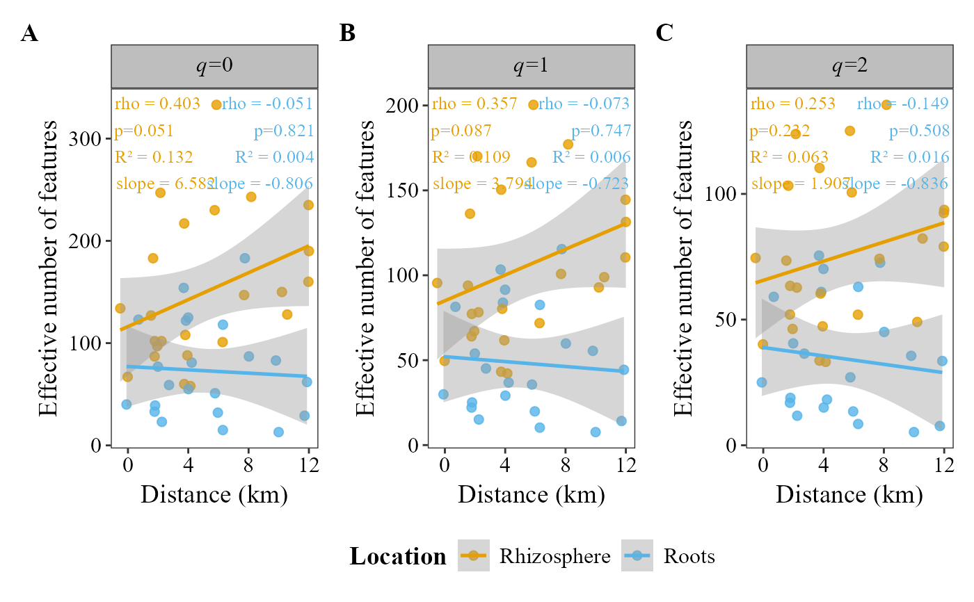
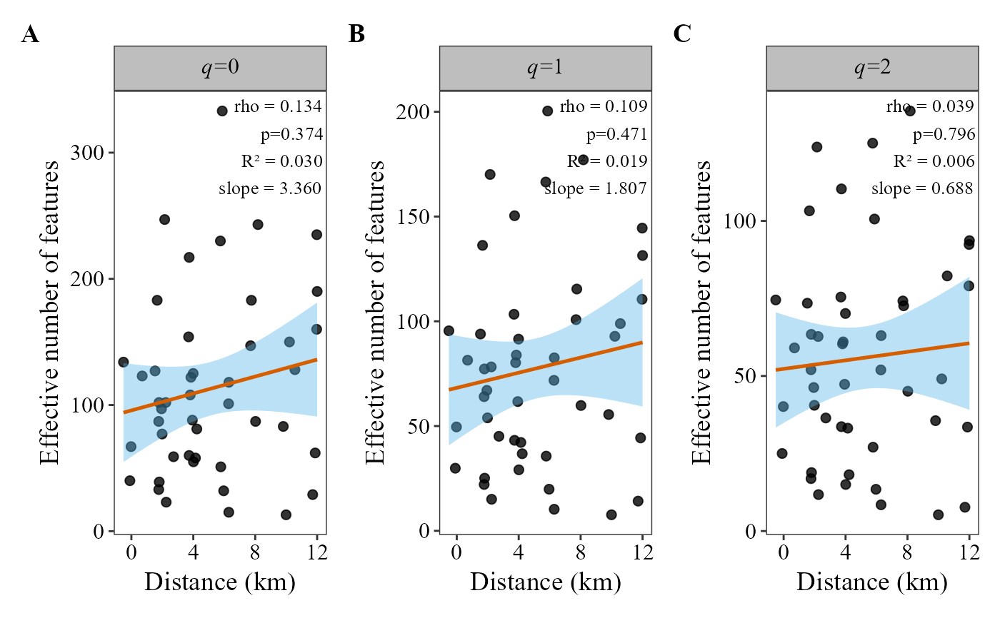
Computes Hill numbers (q = 0, 1, 2) from table and plots them against a continuous metadata variable (e.g. distance to urban center, elevation, pH). It reports the Spearman rank correlation coefficient (rho, or Pearson r), its p-value, and optionally the linear regression \(R^2\) and slope.
Usage
alpha_decay_plot(
  table,
  metadata,
  cont_var,
  group_col = NULL,
  method = "spearman",
  show_lm_stats = TRUE,
  facet_orientation = "horizontal",
  palette = "colorb",
  group_colors = NULL,
  x_axis_title = NULL,
  y_axis_title = "Effective number of features",
  title = NULL,
  show_legend = TRUE,
  legend_position = "bottom",
  free_y = TRUE,
  point_size = 2,
  line_width = 0.9,
  point_alpha = 0.8,
  annotation_size = 3.5,
  panel_label_case = "upper",
  panel_labels = NULL,
  panel_label_bold = TRUE,
  strip_text_bold = FALSE
)
Arguments
- table
A data frame with taxa in rows and samples in columns. The last column must be named
taxonomy, containing full taxonomic strings.- metadata
A data frame containing sample metadata. Its first column must hold the sample IDs (the column names of
table).- cont_var
Character. Name of the continuous variable column in
metadatato place on the x-axis (e.g."dist_km").- group_col
Character. Name of the column in
metadatathat defines the groups, used to color the points and fit one regression line per group. Optional;NULL(default) for no groups.- method
Character. Correlation method for the statistic annotation. One of
"spearman"(default) or"pearson".- show_lm_stats
Logical. If
TRUE(default), adds \(R^2\) and slope from the linear model to the annotation label.- facet_orientation
Character.
"horizontal"(default) puts the three q0/q1/q2 panels in a row;"vertical"in a column.- palette
Character. Palette name:
"colorb"(default, colorblind-friendly Okabe-Ito),"safe"(colorblind-friendly CARTO "Safe"),"earth"(CARTO "Earth", brown to teal; best for two or ordered groups),"grey","viridis"or"brewer".- group_colors
Optional character vector of colors, one per group, named after the groups or in their order. Overrides
palette.- x_axis_title
Character. Title of the x-axis. If
NULL(default), the name ofcont_varis used.- y_axis_title
Character. Title of the y-axis. Default
"Effective number of features".- title
Character. Plot title.
NULL(default) shows no title.- show_legend
Logical. If
TRUE(default), the legend is shown.- legend_position
Character. Position of the legend:
"bottom"(default),"top","right"or"left".- free_y
Logical. If
TRUE, the y-axis scale is free across facets. DefaultTRUE.- point_size
Numeric. Size of the points. Default
2.- line_width
Numeric. Width of regression lines. Default
0.9.- point_alpha
Numeric (0-1). Transparency of the points. Default
0.8.- annotation_size
Numeric. Font size for the stats annotation. Default
3.5.- panel_label_case
Character. Case of the panel tags:
"upper"(default; A, B, C) or"lower"(a, b, c). Ignored ifpanel_labelsis given.- panel_labels
Optional character vector of custom panel tags, one per panel (q0, q1, q2), used as-is (e.g.
c("(a)", "(b)", "(c)")). Overridespanel_label_case.- panel_label_bold
Logical. If
TRUE(default), panel tags are bold. Set toFALSEfor journals that require plain (non-bold) panel tags.- strip_text_bold
Logical. If
TRUE, the facet strip labels are bold. DefaultFALSE.
Value
A patchwork object with the three q0/q1/q2 panels, tagged as
set by panel_label_case or panel_labels. It can still be
modified: p & theme(...) changes every panel, p[[2]] +
labs(...) a single one.
Examples
table_path <- system.file("extdata", "subset_table_bacteria.txt", package = "MicroBioMeta")
table <- read.delim(table_path, row.names = 1, check.names = FALSE)
metadata_path <- system.file("extdata", "subset_metadata_bacteria.txt", package = "MicroBioMeta")
metadata <- read.delim(metadata_path, check.names = FALSE)
loc_dist <- data.frame(Loc = 1:7, dist_km = seq(0, 12, length.out = 7))
metadata$dist_km <- loc_dist$dist_km[match(metadata$Loc, loc_dist$Loc)] +
stats::rnorm(nrow(metadata), sd = 0.3)
# All samples, no grouping. Always tagged A/B/C (see panel_label_case and
# panel_labels to customize)
alpha_decay_plot(
table = table,
metadata = metadata,
cont_var = "dist_km",
x_axis_title = "Distance (km)"
)
#> Warning: cannot compute exact p-value with ties
 # Separate regression lines by location
alpha_decay_plot(
table = table,
metadata = metadata,
cont_var = "dist_km",
x_axis_title = "Distance (km)",
group_col = "Location"
)
#> Warning: cannot compute exact p-value with ties