Hill numbers: taxonomic, phylogenetic and functional diversity
Source:vignettes/hill_diversity.Rmd
hill_diversity.RmdMicroBioMeta computes diversity and returns the figure
ready for publication. This tutorial explains the Hill-number framework
and how to use it in the functions that work with it:
alpha_hill_plot() and alpha_diversity_plot()
for alpha diversity, and beta_ord_plot() and
beta_test_table() for beta diversity. The calculations with
a tree or with traits come from hilldiv3 (Alberdi and Gilbert
2019).
Why Hill numbers
Hill numbers (Hill 1973; Jost 2007) express diversity as an effective number: how many equally abundant taxa would give the same diversity as the sample. A sample with a value of 10 is twice as diverse as one with a value of 5, a statement that does not hold for the Shannon or Simpson indices.
The order sets how much weight the abundances get:
| Order | Weight of the taxa | Equivalent to |
|---|---|---|
| All count the same | Richness | |
| In proportion to their abundance | Exponential of Shannon | |
| Mostly the dominant ones | Inverse of Simpson |
The same idea extends to two other dimensions of diversity (Chao et al. 2014). All three are effective numbers, in species or lineage equivalents (Chao et al. 2021), but they count different things: taxa, lineages or functional groups. Always say which one you report.
diversity |
What it takes into account | What you need | Unit |
|---|---|---|---|
"taxonomic" |
Abundances | The table | Effective number of features |
"phylogenetic" |
How related the taxa are (Chao et al. 2010) | Rooted tree | Effective number of lineages |
"functional" |
How different their traits are (Chao et al. 2019) | Traits per taxon | Effective number of functional groups |
Preparing the data
We use the 18S example of the package (microbial eukaryotes, mostly fungi).
library(MicroBioMeta)

table_fungi <- read.delim(
    system.file("extdata", "table_fungi.txt", package = "MicroBioMeta"),
    row.names = 1, check.names = FALSE
)
taxonomy_fungi <- read.delim(
    system.file("extdata", "taxonomy_fungi.txt", package = "MicroBioMeta"),
    check.names = FALSE
)
metadata_fungi <- read.delim(
    system.file("extdata", "metadata_fungi.txt", package = "MicroBioMeta"),
    check.names = FALSE
)
metadata_fungi <- metadata_fungi[metadata_fungi$SAMPLEID %in% colnames(table_fungi), ]
table_fungi <- table_fungi[, metadata_fungi$SAMPLEID]

table_fung <- merge_feature_taxonomy(table = table_fungi, taxonomy = taxonomy_fungi)
The tree
The tip labels must be the taxa of the table. With QIIME 2 (Bolyen et al. 2019), the tree comes
from the representative sequences, and
exported-tree/tree.nwk is what you read in R:
qiime phylogeny align-to-tree-mafft-fasttree \
    --i-sequences rep-seqs.qza \
    --output-dir phylogeny
qiime tools export --input-path phylogeny/rooted_tree.qza --output-path exported-tree
tree_fungi <- ape::read.tree(
    system.file("extdata", "tree_fungi.nwk", package = "MicroBioMeta")
)
Check the tree before you use it: a few spurious sequences on a very long branch can flatten and , because that branch dominates the tree. In this example we removed three Unassigned ASVs (10 reads) for that reason.
The traits
traits is a table with taxa in rows and traits in
columns. Any measured trait works. For microbial communities a common
source is the table of gene families predicted per ASV by PICRUSt2 (Douglas et al.
2020), such as EC_predicted.tsv. Those are
predictions, not measurements, so report them as such.
traits_fungi <- read.delim(
    system.file("extdata", "traits_fungi.txt", package = "MicroBioMeta"),
    row.names = 1, check.names = FALSE
)
Taxa that are in the table but not in the tree or the traits are dropped with a warning that says how many. Here that happens with the three ASVs above.
Alpha diversity with Hill numbers
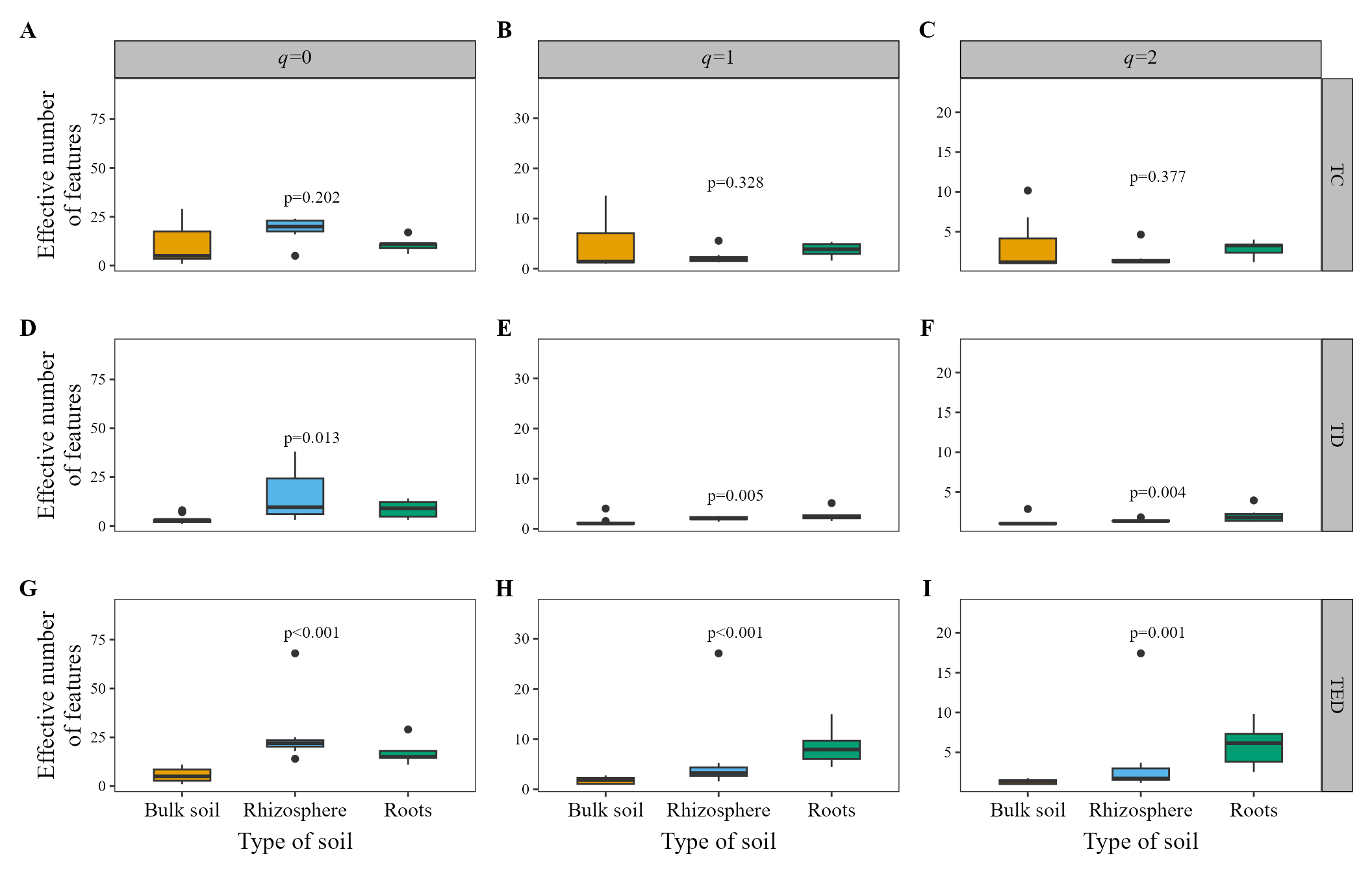
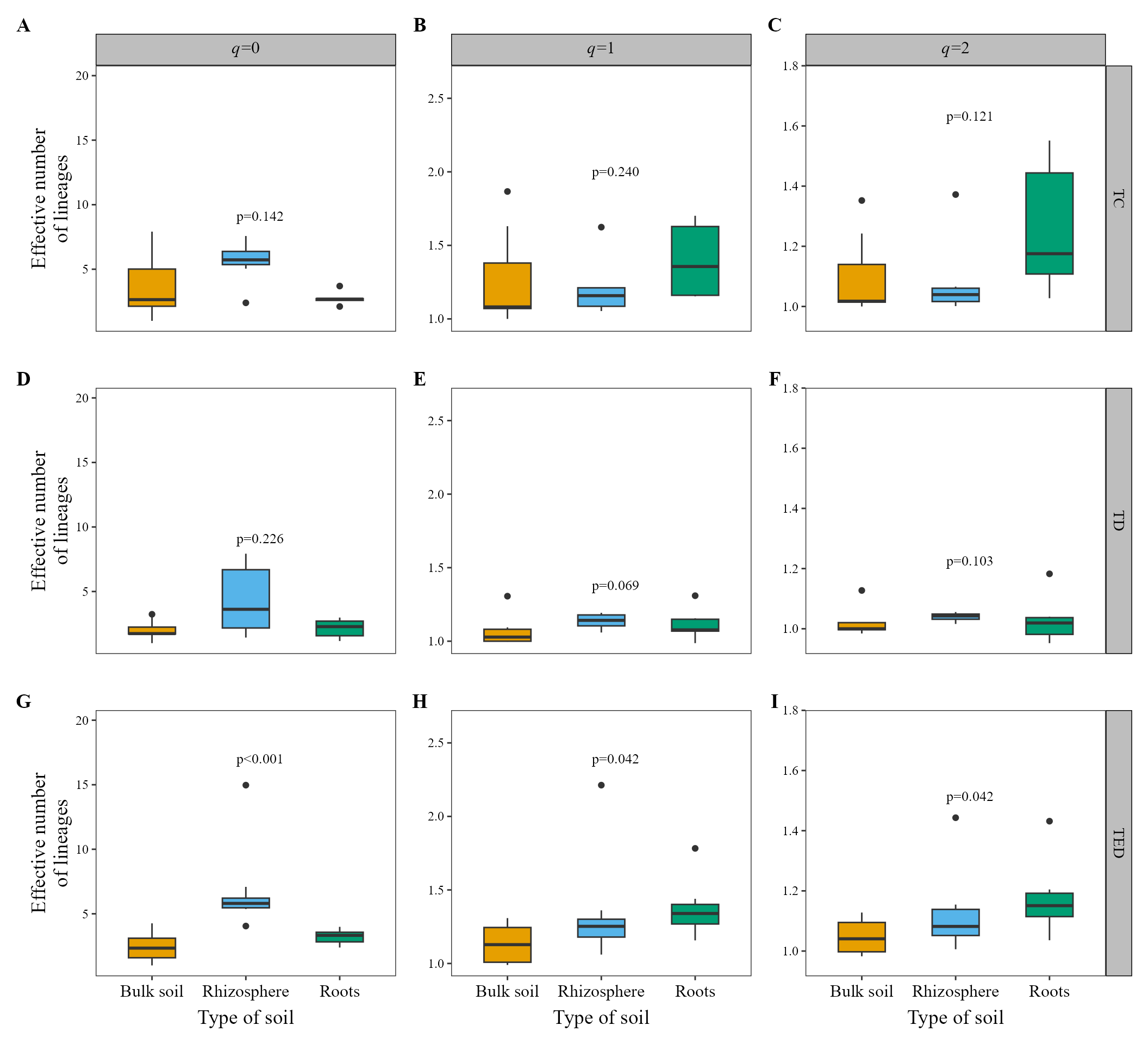
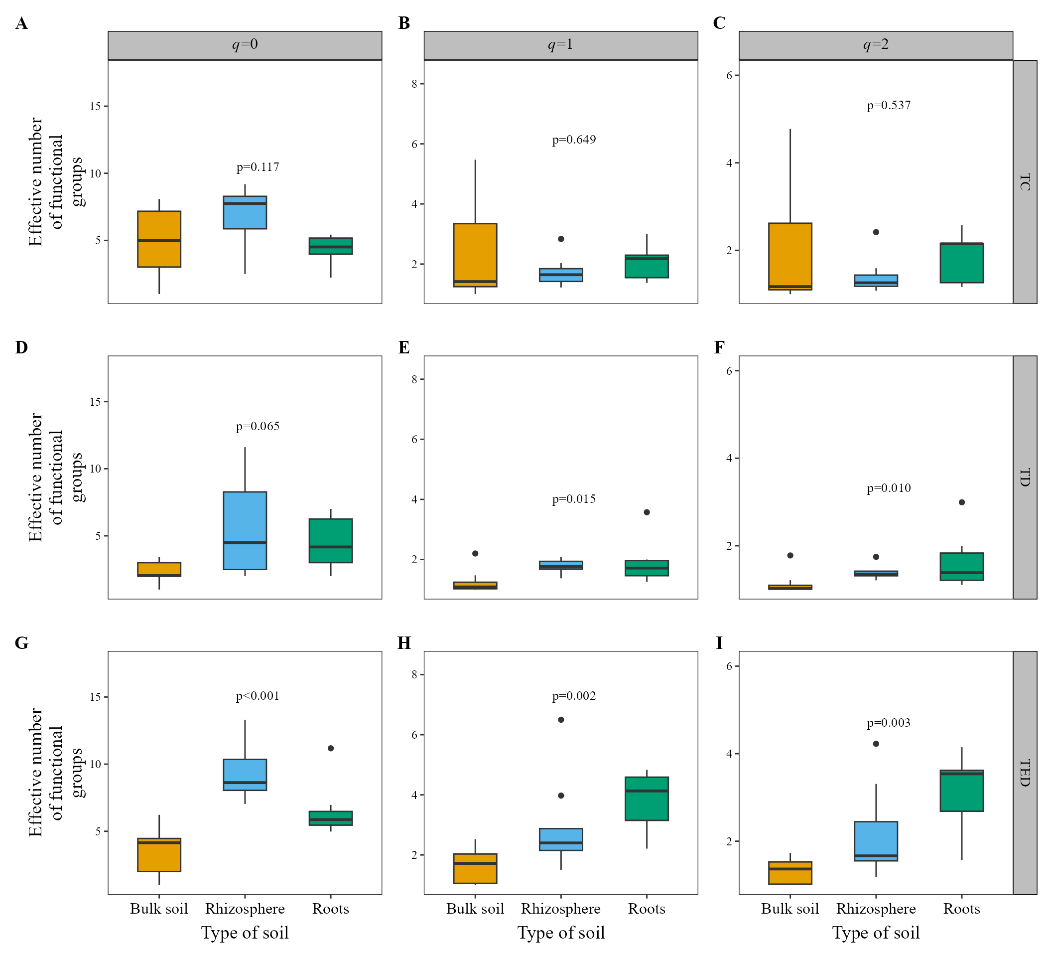
alpha_hill_plot() uses the same call for all three
types. Only diversity and its input change, and the y-axis
title follows the unit of each type.
alpha_hill_plot(
    table = table_fung,
    metadata = metadata_fungi,
    x_col = "Type_of_soil",
    fill_col = "Type_of_soil",
    facet_by = "Treatment",
    x_axis_title = "Type of soil",
    show_legend = FALSE,
    stat = "kruskal.test"
)
alpha_hill_plot(
    table = table_fung,
    metadata = metadata_fungi,
    x_col = "Type_of_soil",
    fill_col = "Type_of_soil",
    facet_by = "Treatment",
    x_axis_title = "Type of soil",
    show_legend = FALSE,
    stat = "kruskal.test",
    diversity = "phylogenetic",
    tree = tree_fungi
)
alpha_hill_plot(
    table = table_fung,
    metadata = metadata_fungi,
    x_col = "Type_of_soil",
    fill_col = "Type_of_soil",
    facet_by = "Treatment",
    x_axis_title = "Type of soil",
    show_legend = FALSE,
    stat = "kruskal.test",
    diversity = "functional",
    traits = traits_fungi
)
Two details of these values:
- The phylogenetic values are read at one common depth, the mean tree
depth of the samples (Chiu et al. 2014), so
samples are comparable. For that reason a sample can fall slightly below
1.
iNEXT.3Duses the age of the root instead, so its values are not the same. - Functional values depend on a threshold
:
taxa at that distance or more count as different functional groups. By
default it is the mean distance between two reads of the pooled samples
(Chao et al.
2019), and you can change it with
tau.
Classic indices
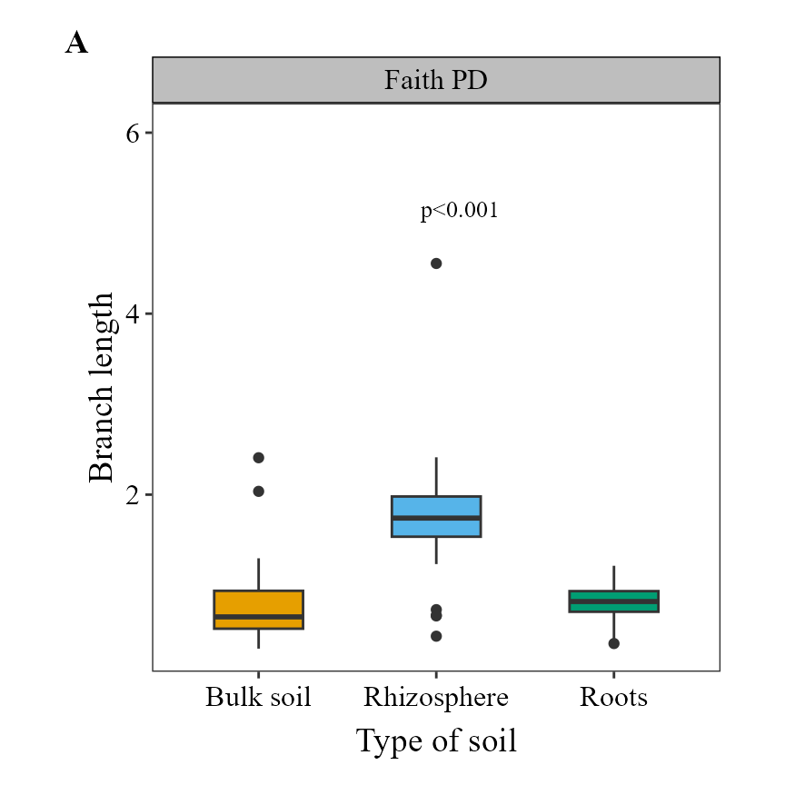
alpha_diversity_plot() shows the classic indices, also
with diversity:
diversity |
Index | Meaning | Unit |
|---|---|---|---|
"taxonomic" |
Chao1, Shannon, Simpson | Richness and evenness | Different in each index |
"phylogenetic" |
Faith’s PD (Faith 1992) | Summed branch length up to the root | Branch length |
"functional" |
Rao’s Q (Rao 1982) | Mean distance between two random reads | Distance (Gower) |
alpha_diversity_plot(
    table = table_fung,
    metadata = metadata_fungi,
    x_col = "Type_of_soil",
    fill_col = "Type_of_soil",
    x_axis_title = "Type of soil",
    show_legend = FALSE,
    stat = "kruskal.test",
    diversity = "phylogenetic",
    tree = tree_fungi
)
alpha_diversity_plot(
    table = table_fung,
    metadata = metadata_fungi,
    x_col = "Type_of_soil",
    fill_col = "Type_of_soil",
    x_axis_title = "Type of soil",
    show_legend = FALSE,
    stat = "kruskal.test",
    diversity = "functional",
    traits = traits_fungi
)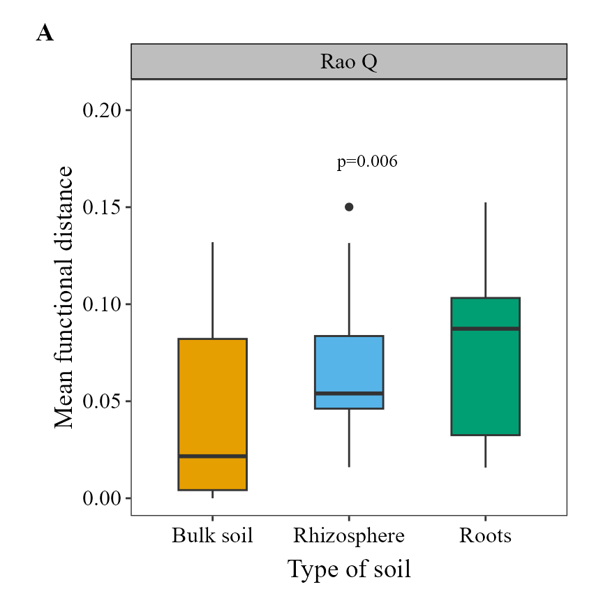
These indices are related to the Hill numbers but they are not the same quantity. Faith’s PD is the phylogenetic before dividing by the depth of the tree, and Rao’s Q gives the functional through when is the largest distance between two taxa. Choose the classic index if you need to compare with studies that report it, and the Hill number if you want every type in the same framework.
Beta diversity
The metrics
hilldiv3::hillpair() turns the Hill numbers into
dissimilarities between samples (Jost 2007; Chiu et al. 2014; Chao et al. 2023). In
MicroBioMeta they are one more option of
distance, next to "jaccard" or
"aitchison", with the order set by q. They
range from 0 (identical samples) to 1 (nothing shared), so they have no
unit problem.
distance |
Type | Taxonomic: , , | Phylogenetic: , , |
|---|---|---|---|
"U" |
Jaccard type | Jaccard, Horn, regional overlap | Phylo-Jaccard (unweighted UniFrac), phylo-Horn, phylo-regional-overlap |
"C" |
Sørensen type | Sørensen, Horn, Morisita-Horn | Phylo-Sørensen (PhyloSor), phylo-Horn, phylo-Morisita-Horn |
"S" |
Jaccard-type turnover | Jaccard, no name, Morisita-Horn | Phylo-Jaccard, no name, phylo-Morisita-Horn |
"V" |
Sørensen-type turnover | Sørensen, no name, no name | Phylo-Sørensen, no name, no name |
The phylogenetic names come from Chiu et al.
(2014), and PhyloSor from
Bryant et al. (2008); UniFrac is from Lozupone and Knight (2005). The functional
versions have no names of their own: Chao et al.
(2019) calls them
Sørensen-type and Jaccard-type functional measures, so report them that
way, with
and
.
At
,
"U" is phylo-Horn, not the weighted UniFrac.
These metrics describe the differences in Hill-number terms; they are not compositional. If your main analysis uses CLR/Aitchison, keep it there and use these as a complement.
Ordination
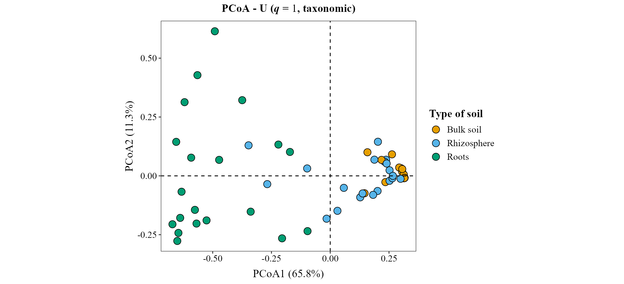
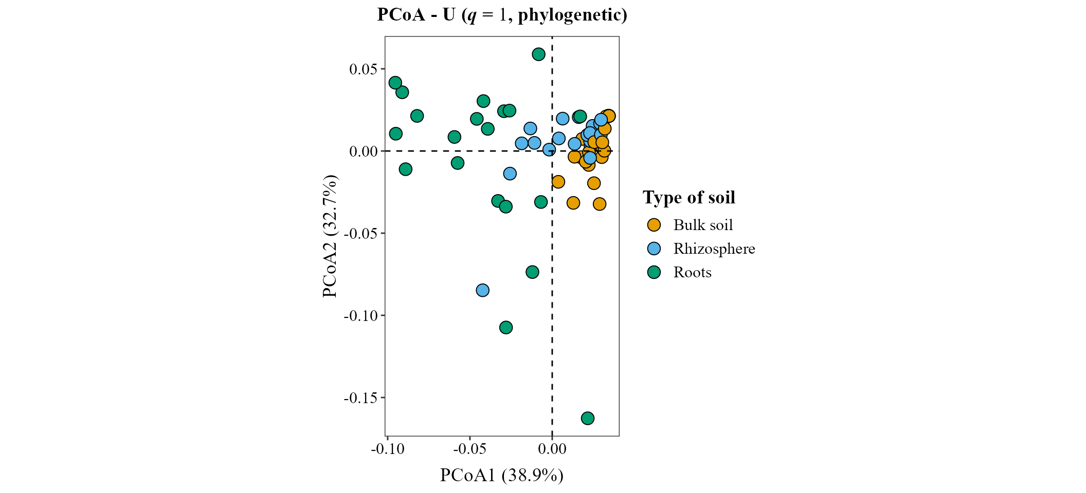
The Hill metrics work with ordination = "PCoA" or
"NMDS", the same as any distance that is not
"compositional". beta_ord_plot() keeps the
same scale on both axes, so the plot gets flat when the first axis
explains most of the variation. In the functional example we add
ggplot2::coord_cartesian() to fill the figure; keep in mind
that the axes no longer share a scale.
beta_ord_plot(
    table = table_fung,
    metadata = metadata_fungi,
    distance = "U",
    q = 1,
    ordination = "PCoA",
    group_col = "Type_of_soil",
    legend_title = "Type of soil"
)
beta_ord_plot(
    table = table_fung,
    metadata = metadata_fungi,
    distance = "U",
    q = 1,
    ordination = "PCoA",
    group_col = "Type_of_soil",
    legend_title = "Type of soil",
    diversity = "phylogenetic",
    tree = tree_fungi
)
beta_ord_plot(
    table = table_fung,
    metadata = metadata_fungi,
    distance = "U",
    q = 1,
    ordination = "PCoA",
    group_col = "Type_of_soil",
    legend_title = "Type of soil",
    diversity = "functional",
    traits = traits_fungi
) + ggplot2::coord_cartesian()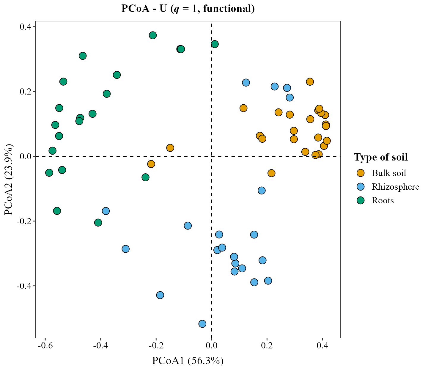
PERMANOVA and betadisper
beta_test_table() takes the same arguments. A PERMANOVA
(Anderson
2001) tests whether the groups differ, and betadisper (Anderson
2006) whether their dispersion does. Report both: a
significant PERMANOVA with unequal dispersions may reflect differences
in dispersion, not in position.
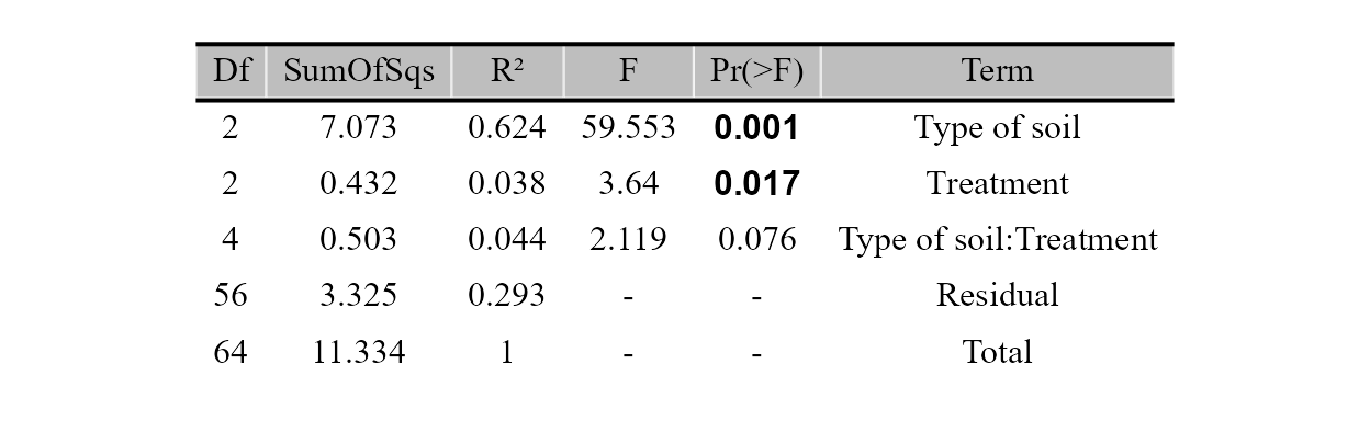
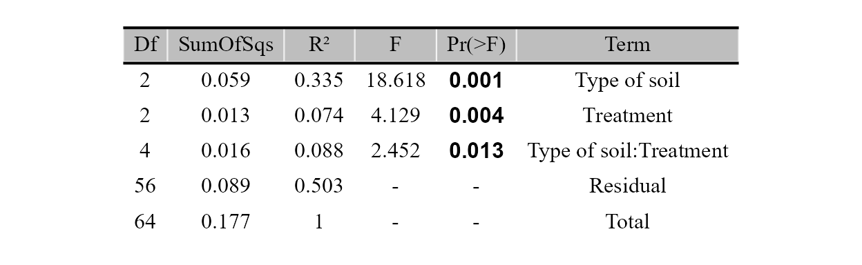
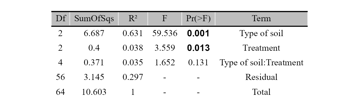
We use and the same model for all three types. At that order soil and treatment differ in all of them, and the interaction only in the phylogenetic one.
Taxonomic:
beta_test_table(
    table = table_fung,
    metadata = metadata_fungi,
    formula_str = "Type_of_soil * Treatment",
    distance = "U",
    q = 1
)
Phylogenetic:
beta_test_table(
    table = table_fung,
    metadata = metadata_fungi,
    formula_str = "Type_of_soil * Treatment",
    distance = "U",
    q = 1,
    diversity = "phylogenetic",
    tree = tree_fungi
)
Functional:
beta_test_table(
    table = table_fung,
    metadata = metadata_fungi,
    formula_str = "Type_of_soil * Treatment",
    distance = "U",
    q = 1,
    diversity = "functional",
    traits = traits_fungi
)
test = "betadisper" works the same way for the three
types. Here is the phylogenetic one. At
the dispersions differ between types of soil in all three, so read the
PERMANOVA of Type_of_soil with that in mind.
beta_test_table(
    table = table_fung,
    metadata = metadata_fungi,
    formula_str = "Type_of_soil",
    distance = "U",
    q = 1,
    test = "betadisper",
    diversity = "phylogenetic",
    tree = tree_fungi
)
References
Session info
## R version 4.6.1 (2026-06-24 ucrt)
## Platform: x86_64-w64-mingw32/x64
## Running under: Windows 10 x64 (build 19045)
##
## Matrix products: default
##   LAPACK version 3.12.1
##
## locale:
## [1] LC_COLLATE=Spanish_Latin America.utf8
## [2] LC_CTYPE=Spanish_Latin America.utf8
## [3] LC_MONETARY=Spanish_Latin America.utf8
## [4] LC_NUMERIC=C
## [5] LC_TIME=Spanish_Latin America.utf8
##
## time zone: America/Mexico_City
## tzcode source: internal
##
## attached base packages:
## [1] stats     graphics  grDevices utils     datasets  methods   base
##
## other attached packages:
## [1] MicroBioMeta_0.99.0
##
## loaded via a namespace (and not attached):
##   [1] deldir_2.0-4                gridExtra_2.3.1
##   [3] permute_0.9-10              rlang_1.3.0
##   [5] magrittr_2.0.5              otel_0.2.0
##   [7] matrixStats_1.5.0           compiler_4.6.1
##   [9] mgcv_1.9-4                  hillR_0.5.2
##  [11] png_0.1-9                   systemfonts_1.3.2
##  [13] vctrs_0.7.3                 stringr_1.6.0
##  [15] pkgconfig_2.0.3             fastmap_1.2.0
##  [17] backports_1.5.1             XVector_0.52.0
##  [19] labeling_0.4.3              rmarkdown_2.32
##  [21] ragg_1.5.2                  purrr_1.2.2
##  [23] xfun_0.61                   Rfast_2.1.5.2
##  [25] randomForest_4.7-1.2        cachem_1.1.0
##  [27] jsonlite_2.0.0              DelayedArray_0.38.2
##  [29] BiocParallel_1.46.0         jpeg_0.1-11
##  [31] broom_1.0.13                parallel_4.6.1
##  [33] cluster_2.1.8.2             R6_2.6.1
##  [35] stringi_1.8.9               bslib_0.12.0
##  [37] RColorBrewer_1.1-3          car_3.1-5
##  [39] zCompositions_1.6.2         GenomicRanges_1.64.0
##  [41] jquerylib_0.1.4             Rcpp_1.1.2
##  [43] Seqinfo_1.2.0               SummarizedExperiment_1.42.0
##  [45] knitr_1.52                  hilldiv3_3.1.1
##  [47] directlabels_2026.8.27      IRanges_2.46.0
##  [49] Matrix_1.7-5                splines_4.6.1
##  [51] tidyselect_1.2.1            dichromat_2.0-1
##  [53] abind_1.4-8                 yaml_2.3.12
##  [55] ggVennDiagram_1.5.7         vegan_2.7-6
##  [57] codetools_0.2-20            lattice_0.22-9
##  [59] tibble_3.3.1                Biobase_2.72.0
##  [61] withr_3.0.3                 S7_0.2.2
##  [63] evaluate_1.0.5              desc_1.4.3
##  [65] survival_3.8-6              RcppParallel_6.2.1
##  [67] pillar_1.11.1               ggpubr_1.0.0
##  [69] MatrixGenerics_1.24.0       carData_3.0-6
##  [71] stats4_4.6.1                NADA_1.6-1.2
##  [73] generics_0.1.4              truncnorm_1.0-9
##  [75] S4Vectors_0.50.3            ggplot2_4.0.3
##  [77] scales_1.4.0                ALDEx2_1.44.0
##  [79] glue_1.8.1                  tools_4.6.1
##  [81] interp_1.1-6                data.table_1.18.6.1
##  [83] ggsignif_0.6.4              ggvenn_0.1.19
##  [85] fs_2.1.0                    cowplot_1.2.0
##  [87] grid_4.6.1                  tidyr_1.3.2
##  [89] ape_5.8-1                   latticeExtra_0.6-31
##  [91] nlme_3.1-169                patchwork_1.3.2
##  [93] Formula_1.2-6               cli_3.6.6
##  [95] zigg_0.0.2                  textshaping_1.0.5
##  [97] S4Arrays_1.12.0             dplyr_1.2.1
##  [99] gtable_0.3.6                ggh4x_0.3.1
## [101] rstatix_1.1.0               sass_0.4.10
## [103] digest_0.6.39               progressr_1.0.0
## [105] BiocGenerics_0.58.1         SparseArray_1.12.2
## [107] ggrepel_0.9.8               htmlwidgets_1.6.4
## [109] farver_2.1.2                htmltools_0.5.9
## [111] pkgdown_2.2.1               lifecycle_1.0.5
## [113] MASS_7.3-65