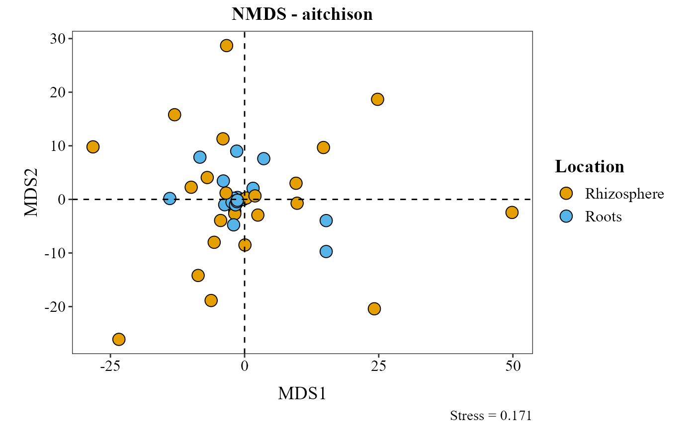
Computes the beta diversity between samples with several distance metrics (including the compositional CLR/Aitchison distance via ALDEx2) and plots a PCA, PCoA or NMDS ordination.
Usage
beta_ord_plot(
  table,
  metadata,
  distance = "compositional",
  mc_samples = 1,
  ordination = "PCA",
  group_col = NULL,
  palette = "colorb",
  shape_col = NULL,
  legend_title = NULL,
  taxonomy_db = "silva",
  arrows_size = 10,
  top_n = 5,
  title = "auto",
  save_table = FALSE,
  table_filename = "ordination_scores.txt",
  q = 1,
  diversity = "taxonomic",
  tree = NULL,
  traits = NULL,
  tau = NULL
)
Arguments
- table
A data frame with taxa in rows and samples in columns. The last column must be named
taxonomy, containing full taxonomic strings.- metadata
A data frame containing sample metadata. Its first column must hold the sample IDs (the column names of
table).- distance
Distance method: one of
"euclidean","bray","jaccard","sorensen","compositional"(default; CLR/Aitchison via ALDEx2),"aitchison","robust.aitchison", or the Hill-number dissimilarities"U","C","V"or"S"ofhilldiv3::hillpair()(with PCoA or NMDS; seeq). Case-insensitive. Note:ordination = "PCA"requiresdistance = "compositional".- mc_samples
Number of ALDEx2 Monte Carlo instances used when
distance = "compositional". With1(default) the clr values of one random instance are used: fast, but the result changes between runs (useset.seed()). With more, the clr values are averaged across instances, which gives an almost identical result in every run;128(ALDEx2's default) is suggested for final analyses, and takes longer. Ignored for other distances.- ordination
Ordination method: one of
"PCA"(default),"PCoA", or"NMDS". Case-insensitive.- group_col
Character. Name of the column in
metadataused to color the points; if it is numeric, a continuous color scale is used. Optional;NULL(default) for no groups.- palette
Either a palette name or a vector of fixed colors; which scale it produces depends on whether
group_colis discrete or continuous.Named, discrete
group_col: one of"colorb"(default; qualitative colorblind-friendly palette),"safe"(colorblind-friendly CARTO "Safe"),"earth"(CARTO "Earth", brown to teal; best for two or ordered groups),"grey","viridis", or"brewer"("Set2").Named, continuous
group_col:"viridis"(default;option = "cividis") or"gradient"Vector of colors, discrete
group_col: used as-is, one color per level (scale_*_manual).Vector of colors, continuous
group_col: used as gradient stops (scale_*_gradientn).
- shape_col
Character. Name of the column in
metadataused for the point shapes. Optional;NULL(default) for one shape.- legend_title
Character. Title of the legend. If
NULL(default), the name ofgroup_colis used.- taxonomy_db
Character. Database the taxonomy strings come from:
"silva"(default),"gg2"(Greengenes2, also"gg"),"unite"or"Kraken2"(also"kraken"). Case-insensitive. Only used whenordination = "PCA".- arrows_size
Numeric. Size/length scaling factor for biplot arrows. Default
10.- top_n
Integer. Number of taxa that contribute most to the PCA, drawn as arrows. Default
5.- title
Character. Plot title.
"auto"(default) shows"Ordination - <distance>";NULLshows no title; any other text is used as the title.- save_table
Logical. If
TRUE, saves the ordination scores and loadings (one table) as a tab-delimited file. DefaultFALSE.- table_filename
Character. Name or path of the saved file (used when
save_table = TRUE). Default"ordination_scores.txt".- q
Numeric. Order of the Hill-number dissimilarities
"U","C","V"and"S": 0 (presence/absence), 1 (default) or 2 (dominant taxa). Ignored by the other distances.- diversity
Character. What the Hill-number dissimilarities use:
"taxonomic"(default),"phylogenetic"(needstree) or"functional"(needstraits). Case-insensitive.- tree
A rooted
phylotree whose tip labels are the taxa oftable. Used whendiversity = "phylogenetic".- traits
A data frame with taxa in rows and traits in columns. Used when
diversity = "functional".- tau
Numeric. Threshold of functional distinctiveness: taxa at this distance or more count as different functional groups.
NULL(default) uses the mean distance between two reads of the pooled samples (Chao et al. 2019). Used whendiversity = "functional".
Details
With distance = "compositional" and mc_samples = 1,
the clr values come from one random Monte Carlo instance of
ALDEx2::aldex.clr(); call set.seed() before the function
to make the result reproducible, or use mc_samples = 128.
Examples
table_path <- system.file("extdata", "subset_table_bacteria.txt", package = "MicroBioMeta")
table <- read.delim(table_path, row.names = 1, check.names = FALSE)

metadata_path <- system.file("extdata", "subset_metadata_bacteria.txt", package = "MicroBioMeta")
metadata <- read.delim(metadata_path, check.names = FALSE)

beta_ord_plot(
    table      = table,
    metadata   = metadata,
    distance   = "aitchison",
    ordination = "NMDS",
    group_col  = "Location",
    top_n      = 5
)
#> Run 0 stress 0.1706715
#> Run 1 stress 0.1882851
#> Run 2 stress 0.2073973
#> Run 3 stress 0.1870265
#> Run 4 stress 0.1943693
#> Run 5 stress 0.1972803
#> Run 6 stress 0.1854032
#> Run 7 stress 0.1848408
#> Run 8 stress 0.1872543
#> Run 9 stress 0.1965079
#> Run 10 stress 0.1972311
#> Run 11 stress 0.1715078
#> Run 12 stress 0.2175272
#> Run 13 stress 0.1942439
#> Run 14 stress 0.1991476
#> Run 15 stress 0.1858242
#> Run 16 stress 0.1848806
#> Run 17 stress 0.1867463
#> Run 18 stress 0.1819661
#> Run 19 stress 0.2076914
#> Run 20 stress 0.1946762
#> Run 21 stress 0.1726581
#> Run 22 stress 0.2012334
#> Run 23 stress 0.1860186
#> Run 24 stress 0.2066487
#> Run 25 stress 0.1873832
#> Run 26 stress 0.1727758
#> Run 27 stress 0.1720405
#> Run 28 stress 0.2186642
#> Run 29 stress 0.1721501
#> Run 30 stress 0.1723186
#> Run 31 stress 0.1782168
#> Run 32 stress 0.1963826
#> Run 33 stress 0.1753228
#> Run 34 stress 0.1827007
#> Run 35 stress 0.2050238
#> Run 36 stress 0.1741984
#> Run 37 stress 0.1899418
#> Run 38 stress 0.1902202
#> Run 39 stress 0.2027131
#> Run 40 stress 0.1885076
#> Run 41 stress 0.1838089
#> Run 42 stress 0.1901196
#> Run 43 stress 0.2039347
#> Run 44 stress 0.1802905
#> Run 45 stress 0.184073
#> Run 46 stress 0.1868212
#> Run 47 stress 0.2102216
#> Run 48 stress 0.2025207
#> Run 49 stress 0.1829283
#> Run 50 stress 0.1788322
#> Run 51 stress 0.1850474
#> Run 52 stress 0.1764492
#> Run 53 stress 0.1949606
#> Run 54 stress 0.189422
#> Run 55 stress 0.1782869
#> Run 56 stress 0.1859456
#> Run 57 stress 0.1837504
#> Run 58 stress 0.1899624
#> Run 59 stress 0.1857217
#> Run 60 stress 0.1981857
#> Run 61 stress 0.1726998
#> Run 62 stress 0.2121562
#> Run 63 stress 0.2129648
#> Run 64 stress 0.186306
#> Run 65 stress 0.2112353
#> Run 66 stress 0.1878251
#> Run 67 stress 0.1796622
#> Run 68 stress 0.1829535
#> Run 69 stress 0.2223803
#> Run 70 stress 0.1982551
#> Run 71 stress 0.1898512
#> Run 72 stress 0.1893261
#> Run 73 stress 0.1981641
#> Run 74 stress 0.1958698
#> Run 75 stress 0.187652
#> Run 76 stress 0.1852827
#> Run 77 stress 0.2071778
#> Run 78 stress 0.1927552
#> Run 79 stress 0.1796531
#> Run 80 stress 0.1803939
#> Run 81 stress 0.2022443
#> Run 82 stress 0.1825395
#> Run 83 stress 0.1791748
#> Run 84 stress 0.1971115
#> Run 85 stress 0.2116146
#> Run 86 stress 0.1796075
#> Run 87 stress 0.174111
#> Run 88 stress 0.208126
#> Run 89 stress 0.1955574
#> Run 90 stress 0.1992225
#> Run 91 stress 0.2081711
#> Run 92 stress 0.1779663
#> Run 93 stress 0.1734975
#> Run 94 stress 0.2137808
#> Run 95 stress 0.2328016
#> Run 96 stress 0.2307386
#> Run 97 stress 0.1873002
#> Run 98 stress 0.1950328
#> Run 99 stress 0.1713901
#> Run 100 stress 0.1949897
#> *** Best solution was not repeated -- monoMDS stopping criteria:
#>     20: no. of iterations >= maxit
#>     80: stress ratio > sratmax
#> Coordinate system already present.
#> ℹ Adding new coordinate system, which will replace the existing one.